Cryptococcus siRNAs
Cryptococcus is one of the few fungi that can become virulent, especially in immunocompromised individuals. Because this fungus has the capacity to grow at temperatures of around 37oC it has been proposed that, apart from a developed immune system, sustaining a high body temperature prevents fungal invasion [Casadevall-2020].
One of the driving forces to develop Coalispr was to create an alternative tool for counting RNA-Seq data obtained for siRNA libraries. We had generated a large number (>100) of such libraries for Cryptococcus deneoformans JEC21 (see About). HTSEQ, the commonly used program to obtain read-counts, required the assembly of an annotation file for siRNA-targets to direct the counting. Small non-coding RNAs have not been annotated, so this had to be done from scratch. A GTF was prepared by manually scanning bedgraph traces in a genome browser like IGB and copying genome coordinates over to a text file and name these regions. From this file a GTF was constructed with a feature useful for counting. Apart from being laborious, this method is error-prone and not very scalable to other organisms or when an update of the genome is published. The counting was also very time-consuming at the time.
This tutorial is based around published data for the related fungus, C. neoformans H99 [Dumesic-2013], [Burke-2019]. As shown below, it can be demonstrated that exons in transcripts, rather than introns [Dumesic-2013], are the target of the RNAi machinery. In C. deneoformans JEC21, siRNAs also align to exons and for both fungi siRNAs crossing splice junctions are identified after mapping with STAR, e.g. at locus CNAG_03231. These findings demonstrate that RNAi acts on spliced transcripts, thus downstream from (instead of parallel to) splicing.
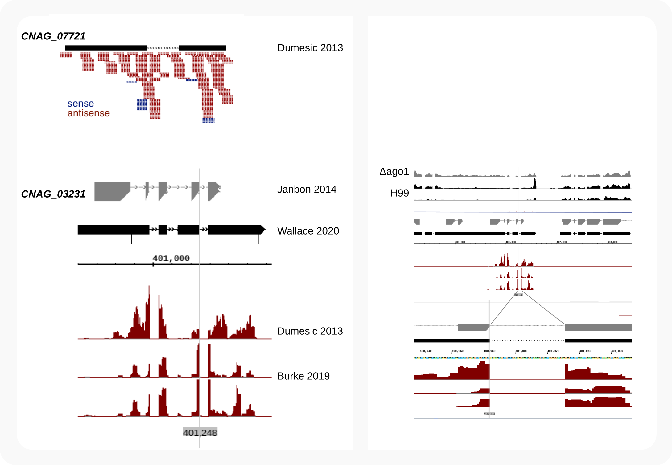
Figure 1. C. neoformans siRNAs target exons, not introns
Compared to other eukaryotes, and possibly related to their ability to grow at 37oC, the GC-content in C. (de)neoformans is very high (~48%). Almost all transcripts carry introns (~98%), often about 5-6 per gene, which appear essential for stable expression [Goebbels-2013], [Janbon-2018]. These unique characteristics [1] make it difficult to predict genes and splicing patterns, which we have encountered when designing tagging strategies. This might also be the reason for the inaccurate model Dumesic et al. put forward in their seminal paper of 2013 [Dumesic-2013]. They proposed that in C. neoformans H99 a pre-mRNA was either spliced or redirected to the RNAi machinery, which was based on the observation that many siRNAs mapped to introns. The annotation file they had used must have been a premature version, as almost all siRNAs actually align to exon sequences described in GTFs published since, including those [2] for the original genomic sequence of this fungus [Janbon-2014]. For example, one of their signature genes, CNAG_07721, has been re-annotated, with the chromosome 8 locus [3] renamed to CNAG_03231.
Bedgraphs, count data accumulated with HTSEQ and hand-made annotations for siRNA loci, supported development of Coalispr and the creation of images for the ‘How-to guides’. This tutorial will show how these images were made. The data will be from publications [Burke-2019] and [Dumesic-2013] which analyzed various genes for their contribution to siRNA accumulation after their disruption with NAT or HYG ([Burke-2019]).
Disrupted Factor |
Reference |
Gene::Marker |
Chromosome |
Strand |
Coordinates |
Short |
|---|---|---|---|---|---|---|
Ago1 |
CNAG_04609::NATR |
|
plus |
|
|
|
Rdp1 |
CNAG_03466::NATR |
|
minus |
|
|
|
Rde1 |
CNAG_01848::NATR |
|
minus |
|
|
|
Rde2 |
CNAG_04954::NATR |
|
plus |
|
|
|
Rde3 |
CNAG_06643::NATR |
|
plus |
|
|
|
Rde4 |
CNAG_01157::NATR |
|
minus |
|
|
|
Rde5 |
CNAG_04791::NATR |
|
plus |
|
|
|
Rrp6 |
CNAG_02773::NATR |
|
minus |
|
|
|
Clr4 |
CNAG_05404_Cterm∆::HYG |
|
plus |
|
|
|
Ezh2 |
CNAG_07553::NATR |
|
minus |
|
|
The organization of reference files will be different from that in the yeast and mouse tutorials. Most downloaded and processed references used for the running of Coalispr are placed in a subfolder, source/, of the work directory.
Note
Outcome of below data-preparation can be downloaded from zenodo.org. See/skip to here
First,
- create a work directory (say, Burke-2019/)
Then, move some files that have been shipped with the program:
copy the contents of this folder in the source distribution: coalispr/docs/_source/tutorials/H99/shared/ to
Burke-2019/.
In a terminal, change directory to the created work environment (from which all scripts and commands will be run):
cd /<path to>/Burke-2019/
Dataset
Following the mouse and yeast tutorials we first generate bedgraph files for C. neoformans data that has been collapsed and uncollapsed. We can obtain bedgraphs after aligning the data to the reference genome. To do this, the raw sequencing data is used and downloaded from the Gene Expression Omnibus (GEO) database with the relevant accession numbers retrieved from the literature:
H99-data |
Reference |
GEO acc. no. |
SRA table |
SRA study |
|---|---|---|---|---|
WT, mutants |
|
|||
WT 2010 |
|
As described for the yeast tutorial:
Open the GEO Accession Display page for the
GSE128009experiment of [Burke-2019].Enter the accession no. into the field
GEO accessionand pressGO.Access
SRA Run Selectorfrom the bottom of the GEO accession display page that has been opened.On the SRA Run Selector webpage, select all
Assay Typelanes formiRNA-Seqand chooseSelectedin theSelectpane.Then click on the
Accession Listbutton in theSelectedrow of theSelectpane.Save the file to the work directory and, because it will be combined with other data, add a prefix.
Save as1_SRR_Acc_List.txt.For detailed info, click the
Metadatabutton for a file describing the experiment.Save asSraRunTable.txt.Do the same for the [Dumesic-2013] sample.
Save theAccession Listfrom theTotalSelectpanel as2_SRR__Acc_List.txt.Save theMetadataas2_SraRunTable.txt.
Collate the lists:
cat 1-SRR_Acc_List.txt 2-SRR_Acc_List.txt > SRR_Acc_List.txt
Download, extract fastq and compress the data (These steps create a directory structure (see Mouse miRNAs) in the working folder the scripts rely on).
sh 0_0-SRAaccess.shThis takes awhile, and so does:sh 0_1-SRAaccess.shsh 0_2-gzip-fastq.sh
Clean and collapse
Adapters present on the reads are removed with:
sh 1_0-flexbar-trim.sh
and a fasta file with collapsed reads is prepared with:
sh 2_0-collapse.sh
Reference traces
Traces for gene-expression in cells can be included in Coalispr. Comparing siRNA signals to mRNA traces is possible because various RNA-Seq datasets are available. Here, we use the bedgraphs prepared by [Wallace-2020] and their annotation file. The reference files will be saved in subfolders of the folder source in the work directory Burke-2019/:
mkdir source
The mRNA reads for parental strain H99 and deletion strains for GWO1 and AGO1 are at GEO accession no. GSE133125 [Wallace-2020]; other samples - not used here - are at GSE206758 [Freitas-2022].
RNA-Seq |
SRA acc. no. |
Run |
Bedgraph |
|---|---|---|---|
H99r1 |
|
|
|
H99r2 |
|
|
|
HdGWO1 |
|
|
|
HdAGO1 |
|
|
Bedgraphs are downloaded and saved to their own folders; you could create these first:
cd sourcemkdir GSM3900523 GSM3900527 GSM3900525 GSM3900529cd ..
Now, for each experiment get the compressed bedgraph files for the PLUS [4] and MINUS strand from the GSM3900523 to GSM3900529 linked pages and save these, ending up with the following folder-hiearchy:
burke-2019
└── source
    ├── GSM3900523
    |   ├── GSM3900523_PN5_index1_ATCACG_L004_R1_001_hisat2_minus.bedgraph.gz
    |   └── GSM3900523_PN5_index1_ATCACG_L004_R1_001_hisat2_plus.bedgraph.gz
    ...
    └── GSM3900529
        ├── GSM3900529_PN10_index18_GTCCGC_L008_R1_001_hisat2_minus.bedgraph.gz
        └── GSM3900529_PN10_index18_GTCCGC_L008_R1_001_hisat2_plus.bedgraph.gz
Then decompress and clean up the files [5]:
for i in source/GSM39*/GSM39*.bedgraph.gz; do gunzip -c $i | sed 's/chr//g' > ${i%.*}
Alignment
Although siRNA reads are expected to be short (~19-24nt) the high density of introns in Cryptococcus makes it feasible that these RNAs can be complementary to regions that cross splice junctions. In other words, it is possible that siRNAs target transcript sections that have undergone splicing. An RNA-focused mapper like STAR can insert gaps that coincide with possible introns when aligning reads to a reference genome. This is the reason why this aligner features in these tutorials.
References
For accurate assignment of introns by STAR it is important to use all information available. One of these resources will be the annotation files describing exons for genes. A second resource is a database of possible splice-junctions that STAR accumulates while alligning reads in an initial pass. Maybe redundant, but we will use both. When generating a genome index, splice-junctions will be retrieved from a recent annotation file; while those found previously on the fly have been collected in a specific file. This file, SpliceJunctionDataBase-sorted-uniq.txt, informs STAR during alignments made in this tutorial. It will also be shown how this file can be updated.
Genome
Download a reference genome for aligning reads to the source/ subfolder:
wget -cN --show-progress -P source "https://ftp.ebi.ac.uk/ensemblgenomes/pub/release-55/fungi/fasta/fungi_basidiomycota1_collection/cryptococcus_neoformans_var_grubii_h99_gca_000149245/dna/Cryptococcus_neoformans_var_grubii_h99_gca_000149245.CNA3.dna_sm.toplevel.fa.gz"
Decompress and simplify seq_id:
gunzip -c source/Cryptococcus_neoformans_var_grubii_h99_gca_000149245.CNA3.dna_sm.toplevel.fa.gz | sed 's/ dna_sm:chromosome [a-z0-9A-Z: ]*$//g' > source/h99.fasta
GTFs
A GFF3 file with transcript annotations used by [Wallace-2020] can be obtained from their github repository:
wget -cN --show-progress -P source "https://github.com/ewallace/CryptoTranscriptome2018/raw/master/CnGFF/H99.10p.aATGcorrected.longestmRNA.2019-05-15.RiboCode.WithStart.gff3
The file has the format of a GTF file with gene-id entries, but gene names can be simplified [6]:
sort -k 1n,1n -k 4n,4n -k 5n,5n source/H99.10p.aATGcorrected.longestmRNA.2019-05-15.RiboCode.WithStart.gff3 | sed 's/"CN[A-N]:/"/g' > source/h99.gtf
The file lacks descriptions for the mitochondria which is obtained below.
To get a reference for non-coding RNAs and pseudo transcripts, get the GenBank annotations
wget -cNrnd --show-progress --timestamping -P source "ftp://ftp.ncbi.nlm.nih.gov/genomes/genbank/fungi/Cryptococcus_neoformans/latest_assembly_versions/GCA_000149245.3_CNA3/GCA_000149245.3_CNA3_genomic.gbff.gz"
Copy coalispr/coalispr/resources/share/genbank2gtf.py to the work folder [7] and run:
python3 genbank2gtf.py -f source/GCA_000149245.3_CNA3_genomic.gbff.gz -p /<path to source folder>/coalispr/coalispr/resources/share/conversion_tables -c H99 -k 4 -o source/ncRNA-pseu.gtf
Get descriptions for the
MTchromosome and add these to the general GTF.
python3 genbank2gtf.py -f source/GCA_000149245.3_CNA3_genomic.gbff.gz -p /<path to source folder>/coalispr/coalispr/resources/share/conversion_tables -c H99 -k 3 -o source/mito.gtfcat source/mito.gtf | sed '1,2d' >> source/h99.gtf
A reference file for counting with HTSeq had been prepared by copy pasting IGB information to a tsv file, source/h99-siRNAsegments.tsv from which a GTF with annotations was created for counting specific reads. In this GTF a specific feature (GTFFEAT) characterizes siRNA segments. The file forms a positive-control reference (GTFSPEC) in Coalispr displays of bedgraph traces. To make this GTF, copy coalispr/coalispr/resources/share/gtf_frm_tsv.py to the work directory (Burke-2019/) and run
python3 gtf_frm_tsv.py -f source/h99-siRNAsegments.tsv -c 2The option-c 2indicates that the input file (-f) relates to H99.
Two other files, h99-xtra.gtf and h99-ncRNAxtra.gtf are shipped with the tutorial that contain additions based on:
possible extraneous DNAs added to the genomes of knockout mutants (i.e. marker genes conferring resistance to nourseothricin (NAT), neomycin/geneticin/G418 (G418) or hygromycin (HYG).
observed differences between data traces and downloaded annotations.
These files will be automatically included when referred to (via GTFXTRA, GTFXTRANAM and GTFUNXTR, GTFUNXTNAM) in the settings file 3.h99.txt and loaded with coalispr showgraphs.
Index
With the annotation file for intron definitions, we can now generate with STAR a genome index for mapping reads to the reference genome. This creates a new folder, the name of which depends on the provided argument. Best practice is that the name for this folder contains EXP, which is set during coalispr init; here we take h99:
sh 3_0-createSTARindex.sh h99
Note that this file import the fasta file with the sequence for the extra annotations as set in h99-xtra.gtf.
The file with chromosome lengths (LENGTHSNAM), created by STAR, can be linked to; place the symbolic shortcut in source/, with other resources for Coalispr:
cd source; ln -sf ../star-h99/chrNameLength.txt h99-chr-lengths.txt; cd ..
Mapping
Map collapsed reads first, this should be fairly quick. Add argument EXP to find the folder with the correct genome information. A second argument would define the number of allowed mismatches; for stringent end-to-end mapping use 0. A third argument can be added to indicate that splice junctions have to be re-recorded from gapped alignments. Set this to 1 if needed; by default this is skipped because such a record comes with the tutorial (also see H99-shared).
sh 3_1-run-star-collapsed-14mer-strict.sh h99 0If splice junction data have been collected [8], prepare the new database with:sh 3_1_1-run-make-SJDB.sh h99
If this all finishes ok, map the uncollapsed data; by default the available database of spliced junctions will be used.
sh 4_1-run-star-uncollapsed-14mer-strict.sh h99[9]
Then, bedgraphs can be made. The scripts take two parameters, for EXP and the number (0 by default) of mismatches.
sh 3_2-run-make-bedgraphs.sh h99sh 4_2-run-make-bedgraphs-uncollapsed.sh h99
For quality control information, the following script (with the same two parameters) is available:
sh 5_1-QC-reports.sh h99
- As a check for the mapping we inspect in a genome browser the accumulation of cDNAs, i.e. the collapsed data, at the CNAG_03231 locus on chromosome 8. The number of sense cDNAs is in a comparable range as the antisense cDNAs, but far more copies of antisense siRNAs are expressed as shown in Figure 1 where the uncollapsed sense signals are not coming above the base line.
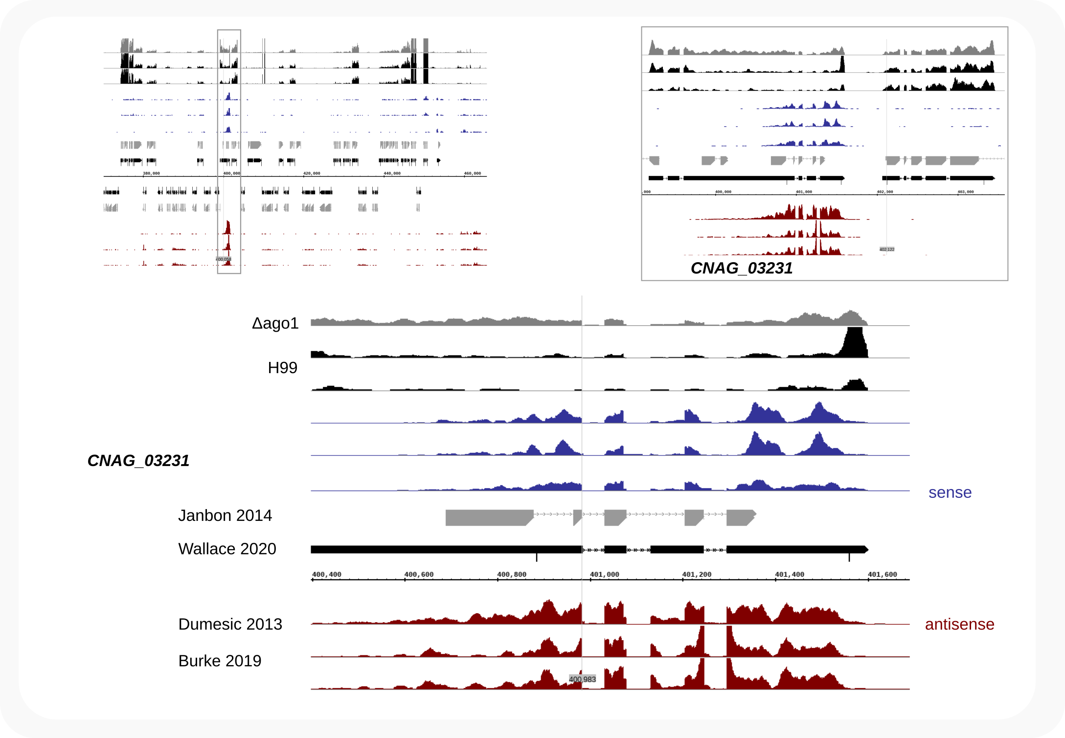
Figure 2. C. neoformans siRNA cDNAs target exons, not introns
Note
Datasets prepared above were uploaded to zenodo.org (DOI 10.5281/zenodo.12822543). These can also be used for testing Coalispr.
cd <path to workfolder>wget -cNrnd --show-progress --timestamping "https://zenodo.org/records/12822544/files/Burke-2019.tar.gz?download=1"tar -xvzf Burke-2019.tar.gz
Updated versions of Coalispr may require new configuration files, please check the zenodo site. Download and extract the archive Replacement_files_for_Coalispr-$VERSION.tar.gz, then copy the relevant files/folders over to the Coalispr directory in the workfolder.
Coalispr
The input materials, the bedgraph files, are available. The analysis begins with setting up the program for this experiment (EXP), which will be named to h99.
cd /<path to>/Burke-2019coalispr initbash-5.2$ coalispr init Please provide a name for this new session/experiment. This name will be used in commands and in file paths. (therefore best to keep it short and memorable, without spaces or special characters). Experiment name: ('stop' to cancel) h99 Experiment name will be set to: 'h99' Is that OK? 1: Yes 2: Cancel ?: 1 Experiment name has been set to 'h99'. Now, set the work folder for this session/experiment. Files are stored in folder 'Coalispr' either in the user's home directory, or in the current folder (before running the `init` command, change directory to this destination first). Alternatively keep files near the source code, in the coalispr installation folder. (The directory with the installation folder will be shown as option in this case.) Configuration files, figures and data go in sub-folders: 'constant_in' for configuration files, 'figures', and 'data' for storage of binarized input and count files. Please choose a folder. ('stop' to cancel) 1: home (rob) 2: current (Burke-2019) 3: source (COALISPR) Enter an option: 2 Path to Coalispr folder will be set to: '/<path to>/Burke-2019/Coalispr' Is that OK? 1: Yes 2: Cancel ?: 1 Configuration files to edit are in: '/<path to>/Burke-2019/Coalispr/config/constant_in' The path '/<path to>/Burke-2019/Coalispr' will be set as 'SAVEIN' in 3_h99.txt.
Configuration
Explained in the How-to guides is the preparation of configuration files with settings, especially the 3_EXP.txt, and the file (EXPFILE) describing the data for the experiment.
Note
When using the alignments downloaded from zenodo.org, the EXPFILE, /<path to>/Burke-2019/source/h99-experiment_table.tsv, is ready and only the shipped configuration file /<path to>/Burke-2019/Coalispr/constant_in/3_h99_zenodo.txt needs to be adapted to your local setup:
From
3_h99.txtcreated bycoalispr init, copy relevant [12] values for:SETBASE
SAVEIN (BASEDIR / PRGNAM).
and replace those in
3_h99_zenodo.txtRemove/rename
3_h99.txtRename/link
3_h99_zenodo.txtto3_h99.txt
Experiment file
The file describing the experiment has been assembled from the SraRunTable.txt for the two GEO datasets as follows:
Short   Run       Category  Method   Group  Fraction  Condition  Read-density  Experiment  Variation  GEO_Accession (exp)  DOI
wt_0    SRR646636      S    total             WCE                   NaN        SRX215659    WT 2010      GSM1061025        10.1016/j.cell.2013.01.046
a1_1    SRR8697580     U    total    a1       WCE                   NaN        SRX5493436    ago1        GSM3660325        10.25387/g3.7829429
a1_2    SRR8697581     U    total    a1       WCE                   NaN        SRX5493437    ago1        GSM3660326        10.25387/g3.7829429
c4_1    SRR8697582     M    total    meth     WCE                   NaN        SRX5493438    clr4        GSM3660327        10.25387/g3.7829429
c4_2    SRR8697583     M    total    meth     WCE                   NaN        SRX5493439    clr4        GSM3660328        10.25387/g3.7829429
e2_1    SRR8697584     M    total    meth     WCE                   NaN        SRX5493440    ezh2        GSM3660329        10.25387/g3.7829429
e2_2    SRR8697585     M    total    meth     WCE                   NaN        SRX5493441    ezh2        GSM3660330        10.25387/g3.7829429
re1_1   SRR8697586     M    total    re1      WCE                   NaN        SRX5493442    rde1        GSM3660331        10.25387/g3.7829429
re1_2   SRR8697587     M    total    re1      WCE                   NaN        SRX5493443    rde1        GSM3660332        10.25387/g3.7829429
re2_1   SRR8697588     M    total    re2      WCE                   NaN        SRX5493444    rde2        GSM3660333        10.25387/g3.7829429
re2_2   SRR8697589     M    total    re2      WCE                   NaN        SRX5493445    rde2        GSM3660334        10.25387/g3.7829429
re3_1   SRR8697590     M    total    re3      WCE                   NaN        SRX5493446    rde3        GSM3660335        10.25387/g3.7829429
re3_2   SRR8697591     M    total    re3      WCE                   NaN        SRX5493447    rde3        GSM3660336        10.25387/g3.7829429
re4_1   SRR8697592     M    total    re4      WCE                   NaN        SRX5493448    rde4        GSM3660337        10.25387/g3.7829429
re4_2   SRR8697593     M    total    re4      WCE                   NaN        SRX5493449    rde4        GSM3660338        10.25387/g3.7829429
re5_1   SRR8697594     M    total    re5      WCE                   NaN        SRX5493450    rde5        GSM3660339        10.25387/g3.7829429
re5_2   SRR8697595     M    total    re5      WCE                   NaN        SRX5493451    rde5        GSM3660340        10.25387/g3.7829429
r1_1    SRR8697596     U    total    r1       WCE                   NaN        SRX5493452    rdp1        GSM3660341        10.25387/g3.7829429
r1_2    SRR8697597     U    total    r1       WCE                   NaN        SRX5493453    rdp1        GSM3660342        10.25387/g3.7829429
r6_1    SRR8697598     M    total    r6       WCE                   NaN        SRX5493454    rrp6        GSM3660343        10.25387/g3.7829429
r6_2    SRR8697599     M    total    r6       WCE                   NaN        SRX5493455    rrp6        GSM3660344        10.25387/g3.7829429
wt_1    SRR8697600     S    total             WCE                   NaN        SRX5493456    Kn99alpha   GSM3660345        10.25387/g3.7829429
wt_2    SRR8697601     S    total             WCE                   NaN        SRX5493457    Kn99alpha   GSM3660346        10.25387/g3.7829429
h99_1   GSM3900523     R    rnaseq                                  1          SRX6102296    RNA_H99r1   GSM3900523        10.1093/nar/gkaa060
h99_2   GSM3900527     R    rnaseq                                  4          SRX6102300    RNA_H99r2   GSM3900527        10.1093/nar/gkaa060
h99-a1  GSM3900529     R    rnaseq                                  5          SRX6102302    RNA_HdAGO1  GSM3900529        10.1093/nar/gkaa060
h99-g1  GSM3900525     R    rnaseq                                  2          SRX6102298    RNA_HdGWO1  GSM3900525        10.1093/nar/gkaa060
For columns METHOD, FRACTION or GROUP only values relating to particular methods, fractions or conditions are filled in. When one value applies to all samples it can be omitted; but then the group will not be shown in coalispr showgraphs. Thus, in the example above, METHOD and FRACTION will be visible but CONDITION will not be indicated. The numbers in the Read-density (READDENS) column for the mRNA references lead to an adaptation of the traces so that their overall display is at a comparable level. This can be done because the expression of most transcripts do not seem to be affected by the deletions. In other words, it is an application of the principle guiding normalization when differential expression of genes is assessed (see About) [10]. Adjusting the relative Read-density makes it easier to observe putative effects of the absence of Ago1 or Gwo1 on expression of transcripts targeted by siRNAs.
Settings file
For the configuration, in the file 3_h99.txt (copied from 3_EXP.txt in the init step) the following fields [11] were set to the given values:
EXP : “h99” [12]
CONFNAM : “3_h99.txt” [12]
EXPNAM : “C. neoformans”
UNSPECLOG10 : 0.78
MAXGAP : 400
XLIM0 : 14
XLIM1 : 36
XLIM00 : 18
SETBASE : “/<path to>/Burke-2019/”
REFS : SOURCE
EXPFILNAM : “h99-experiment_table.tsv”
RIP1 : “”
RIP2 : “”
NOTAGIP : “”
- MUTGROUPS{
- “a1”:”ago1\u0394”, “re1”:”rde1\u0394”, “re2”:”rde2\u0394” [13]“re3”:”rde3\u0394”, “re4”:”rde4\u0394”, “re5”:”rde5\u0394”,“r1”:”rdp1\u0394”, “r6”:”rrp6\u0394”, OTHR:”methyl\u0394”,}
- FRACTIONS{
- WCE:”Cell extract”,}
- UNSPECIFICS[
- “a1”, “r1”,]
- MUTANTS[
- “re1”, “re2”, “re3”, “re4”, “re5”, “r6”, OTHR,]
LENGTHSNAM : “h99-chr-lengths.txt”
DNAXTRNAM : “NAT_G418_HYG.fa”
LENXTRA : “7062”
CHRXTRA : XTRA
GTFSPECNAM : “h99-siRNAsegments.gtf”
GTFUNSPNAM : “ncRNA-pseu.gtf”
GTFREFNAM : “h99.gtf”
GTFXTRANAM : “h99-xtra.gtf”
GTFUNXTNAM : “h99-ncRNAxtra.gtf”
# SAVEIN : Path(“/<path to>/Burke-2019/Coalispr”) [12]
SAVEIN : BASEDIR / PRGNAM [14]LENGTHSFILE : BASEDIR / SOURCE / LENGTHSNAM
DNAXTRA : BASEDIR / SOURCE / DNAXTRNAM
EXPFILE : BASEDIR / SOURCE / EXPFILNAM
GTFSPEC : BASEDIR / SOURCE / GTFSPECNAM
GTFUNSP : BASEDIR / SOURCE / GTFUNSPNAM
GTFREF : BASEDIR / SOURCE / GTFREFNAM
GTFXTRA : BASEDIR / SOURCE / GTFXTRANAM
GTFUNXTR : BASEDIR / SOURCE / GTFUNXTNAM
Analysis
Bedgraph data are loaded and compared in Coalispr by means of Pandas dataframes. For repeated use, the data are stored in a binary (parquet) format that is common and exchangeable. The coalispr storedata steps below accomplish this.
Note
When using the archive with alignments downloaded from zenodo.org, otcomes of this step can be compared to binary, processed data that come with the archive to test commands like coalispr showgraphs or coalispr countbams.
Store uncollapsed, then collapsed data (-t1), while processing both data (-d1) and reference (-d2) bedgraph files.
coalispr storedata -d1coalispr storedata -d2coalispr storedata -d1 -t1coalispr storedata -d2 -t1
Example output of last run, skipping files already processed.
bash-5.2$ coalispr storedata -d2 -t1
Logger coalispr.coalispr started...

Processing references ...

Samples have been merged before; no bedgraphs to process.
 To redo, rename/remove reference_merged.

References were specified in relation to collapsed reads.

Finished 'process_reference' in 0.73 secs
Most messages written to the terminal also end up in the log file in /Burke-2019/Coalispr/logs/h99/. Check the logs to get an idea about the involved steps. Further, files are saved for use by other parts of the program based on the threshold UNSPECLOG10 (of 0.78; representing a minimal ~6 fold difference in the case of overlapping signals for SPECIFIC/MUTANT samples vs. UNSPECIFIC samples in bins marked by the indices).
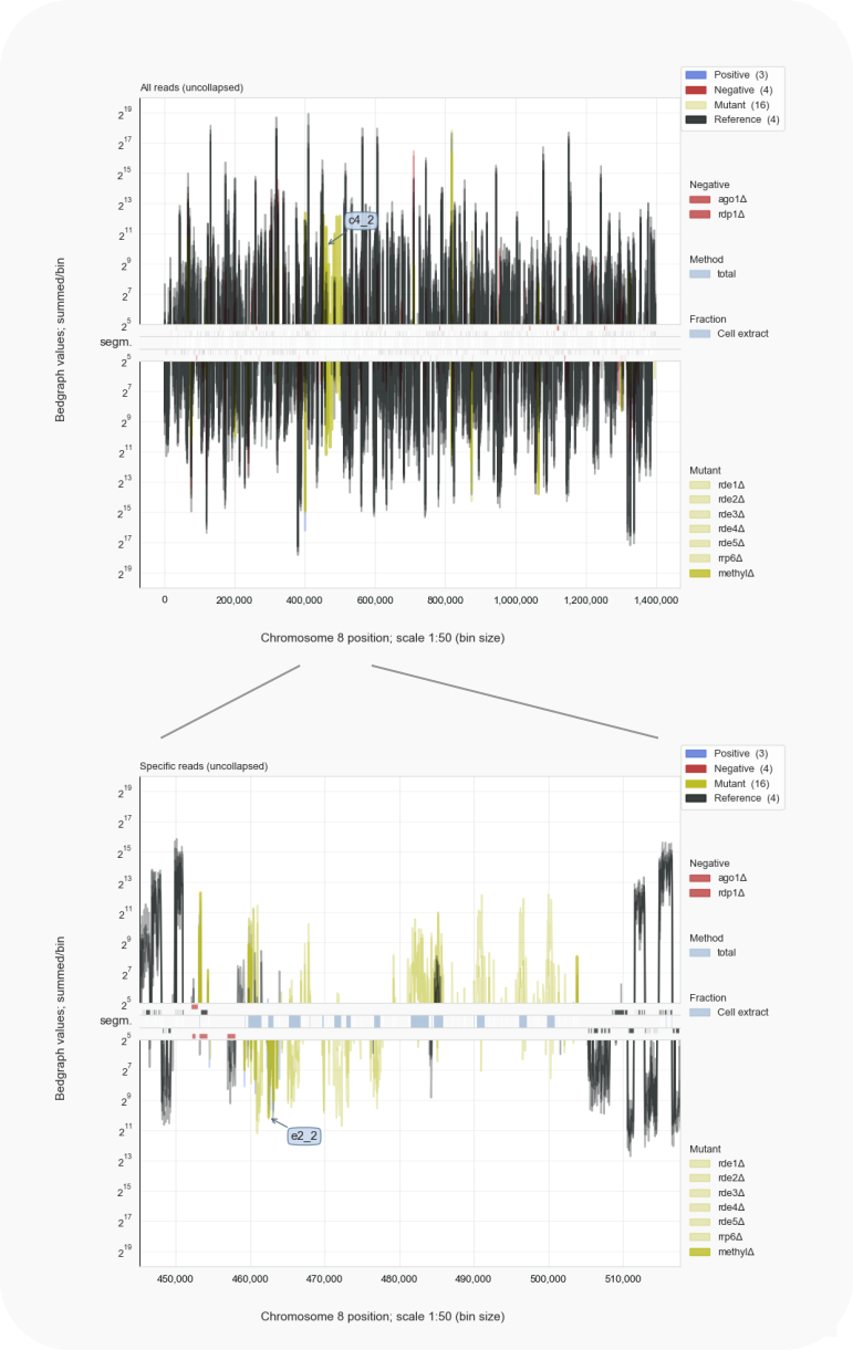
Figure 3. Visualization of centromeres.
Normally, centromeres are not transcribed, as indicated by the gap in mRNA transcripts (black). Inactivation of histone H3 methylation by deletions in genes for Clr4 (c4) or Ezh2 (e2) leads to loss of silencing of centromeric transcripts to which siRNAs are raised [Burke-2019]. With: coalispr showgraphs -c 8 -w2.
Graphs
Check traces:
coalispr showgraphs -c 8 -w2
Proteins involved in methylation of DNA and of histone H3, leading to heterochromatin formation and thereby silencing of genes in these chromosome regions, are important to reduce the production of siRNAs complementary to transcripts expressed from centromeres [Burke-2019]. Centromeres in Cryptococcus are long and consist of repetitive DNA derived from transposable elements [1]. The length of centromeres, together with the absence of RNAi against transposons in an organism, appears related to virulent behaviour of fungi [Yadav-2018]. The results from [Burke-2019] are helping to light up centromeric regions in bedgraph displays by Coalispr.
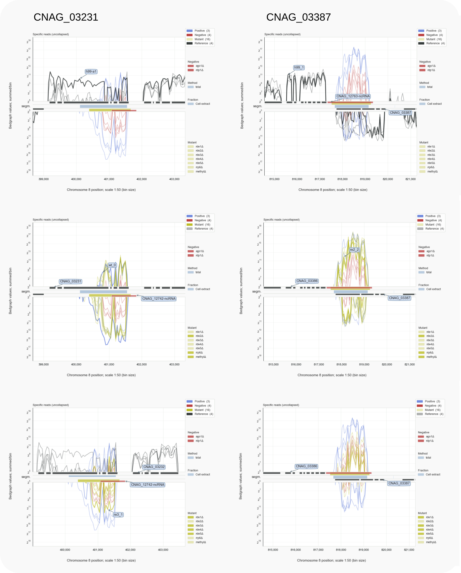
Figure 4. CNAG_03231 and CNAG_03387
Segments representing an siRNA locus have been annotated as a ncRNA. Not all mutants have an equal effect on siRNA formation. One group appears as wild type (middle) and another as the negative controls (bottom). Traces for Specific reads are shown (with: coalispr showgraphs -c8 -w4).
To revisit CNAG_03231, and see the impact of mutants on siRNA formation (see Fig. 4, run:
coalispr showgraphs -c8 -w4
And zoom in to regions 399000-403600 for CNAG_03387 or 814700-821200 for CNAG_03387. Alternatively, using the region option -r, for CNAG_03387 run:
coalispr showgraphs -c8 -w4 -r 399000-403600
For CNAG_03387:
coalispr showgraphs -c8 -w4 -r 814700-821200
This will show traces after filtering out the unspecific reads [15]. The C-terminal encoding regions of the transcripts are targeted by siRNAs. That introns have been removed by splicing is better visible in a genome browser; the 50-fold reduced resolution in the Coalispr display can only hint at this. Note that in absence of RNAi (in the h99-a1 mutant lacking Ago1) relatively higher mRNA expression levels are detectable for these loci compared to wild type (h99) and surrounding loci.
In the other tutorials, to support the article , rDNA loci have been analyzed.
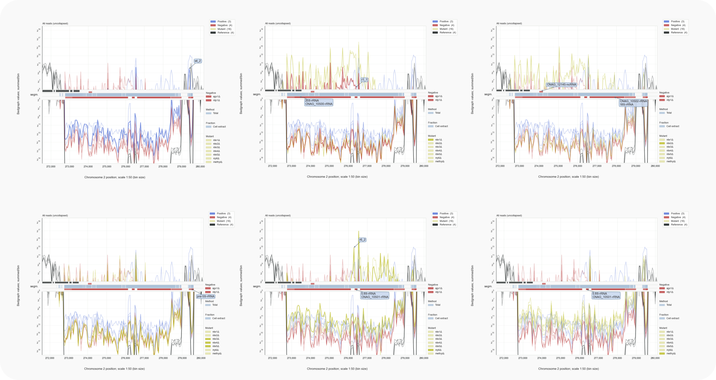
Figure 5. C. neoformans rDNA locus [16]
Reads representing rRFs are abundant in all samples to a comparable extent. In some clones, but not all, reads complementary to rRNA are formed. For the rde1Δ (top mid) and rde2Δ (top right) strains these reads counter regions of large subunit rRNAs 25S and 5.8S, while in wild type (top left) or rrp6Δ (bottom mid) the small subunit 18S rRNA region and flanking transcribed spacers are targeted. No effect is visible for strains lacking Rde3, Rde4 or Rde5 (bottom left) or in strains without DNA or histone methylation activity (bottom right). Although a contamination with rDNA might have caused this, the signals are typical for the strains and could have another source of origin. Note the rRNA peaks of the reference RNA-Seq libraries that run off the scale (black). Traces for all reads are shown (with: coalispr showgraphs -c2 -w2 ).
In Cryptococcus the rDNA is on chromosome 2, on the minus strand. All reads are shown with:
coalispr showgraphs -c2 -w2Using the
zoomtool, exposes the rDNA region from270000to284000
This command produces a display of traces that shows that rRFs are common to all samples. In some strains, including the wild type (from [Dumesic-2013]), reads are mapped that are antisense to the rRNA. Can these be the result of an RNAi response? Or are they generated by another, possibly artefactual mechanism?
Add count data
To obtain a more detailed insight in the kind of reads in the various libraries, we start with getting count data.
Counts for the input:
coalispr countbams -rc 1(for uncollapsed data)coalispr countbams -rc 2(for collapsed data)
Counts for aligned reads:
coalispr countbams(for specific data)coalispr countbams -k0 -u 1
With this information, we can inspect cDNA traces (of collapsed reads) with siRNA-like lengths and start-nucleotide [17] that are present in the negative data:
coalispr showgraphs -c2 -t1
This shows that such common small RNAs can derive from highly expressed transcripts (top left panel in the figure, including rRNA. Fitting the finding that siRNA populations consist of sense and antisense reads, such small RNAs are found to map to the rDNA, although mostly in a similar manner as found for the negative control lacking Rrp1 (r1). A fraction of reads that does not overlap with negative control reads is found in the wild type and a strain with mutant RRP6. Does this mean that rRFs are actually part of the siRNA population associated with Ago1 in a biologically relevant manner? Or is it that rRNA, rather than supplier, becomes a target of RNAi? Because of the mix-up with rRNA as common contaminant and the possibility that unselected siRNAs obtained their features by chance, these questions cannot be answered on the basis of these observations. For example, there is no idea about the length-distributions of the mapped reads; do the siRNA-like reads stand out from the remainder? This question is answered below.
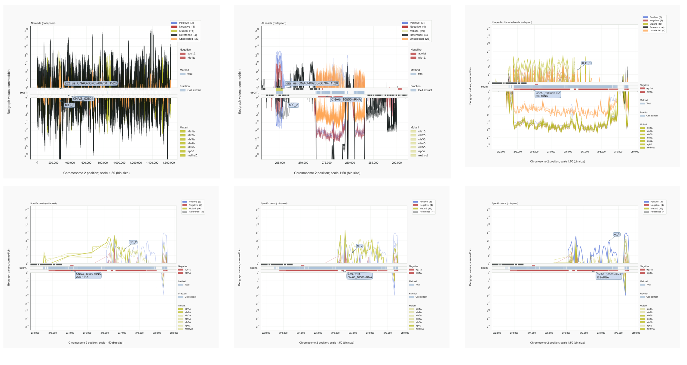
Figure 6. C. neoformans rDNA locus [16], mapped cDNAs.
cDNAs of unselected reads adhere to siRNA characteristics but fall in the class of unspecific sequences due to an overlap with common signals found in negative control samples. Many of these reads derive from highly expressed transcripts (orange traces on top of black mRNA signals, top left). This is also the case for the DNA regions with genes for rRNA (top middle), although a diverse population of cDNAs is found to be anti-sense to 25S and 5.8S or 18S rRNAs, which is also observed for the negative control lacking a functional RRP1 gene (top right). Anti-sense cDNAs against the 18S rRNA region and flanking transcribed spacers are specific for the wild-type strain or seen in the absence of Rrp6 (bottom) (with: coalispr showgraphs -c2 -t1 ).
Count diagrams
Coalispr is a tool to check libraries in a data set, and obtain counts for specified reads as done above. How different are the libraries with respect to coverage and number of mapped reads? For this, we can look at the uncollapsed and collapsed reads, respectively, using alignment information:
coalispr showcounts -rc 1coalispr showcounts -rc 2
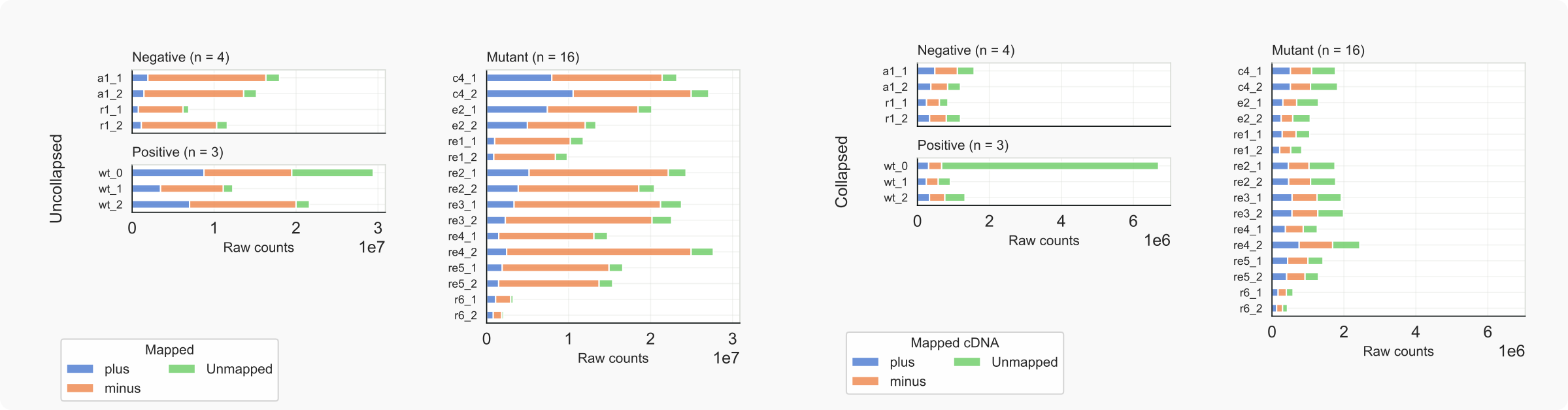
Figure 7. C. neoformans libraries, mapped (stranded) vs. unmapped reads.
According to these diagrams, the libraries are fairly comparable although the original data (wt_0) [Dumesic-2013] contain a high number of unmapped reads, possibly due to adapter remnants that interfere with the stringent EndToEnd mapping [9]. In general the background is fairly high. This observation is based on the overlap between the positive and negative control samples, with respect to a) the large fraction of common minus-strand reads (the rDNA gene is on that strand on chromosome 2) in the positive and mutant samples, while b) negative control samples contain reads that are specified as specific [18]. The characteristics for the libraries of mutant rde1Δ (re1) are very similar to that of the negative controls, suggesting that RNAi has been inactivated in the absence of Rde1. The strains lacking Rrp6 (r6) yielded a relatively low number of reads. According to Burke et al [Burke-2019] for all samples 20 μg RNA was used for library preparation of siRNAs. Assuming that experimental parameters for library preparation were comparable, are the low siRNA yields for rrp6Δ strains indicative for a poor state of these cells (slow growth, reduced RNA synthesis or minimal RNAi activity)?
Checking the overall counts for specific and unspecific reads gives other information:
coalispr showcounts -lc {1-7}
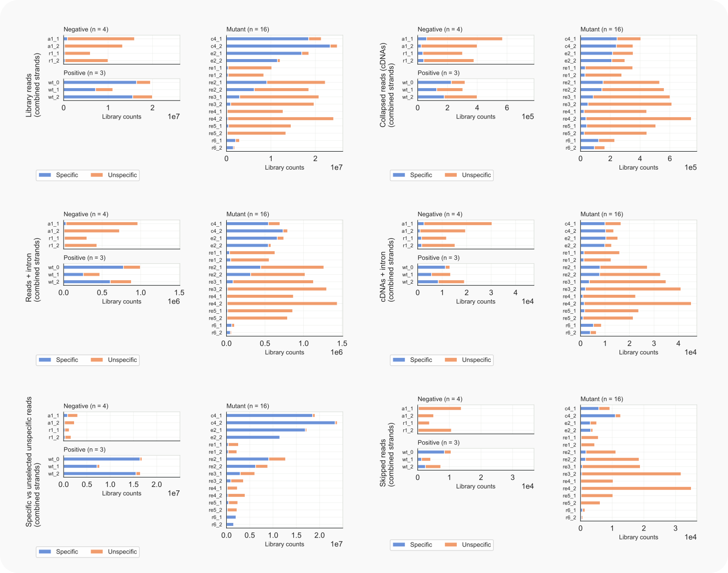
Figure 8. C. neoformans library counts, specific vs. unspecific reads.
-lc 1; left) and collapsed data, cDNAs (-lc 2; right).-lc 4; left), and in cDNAs (-lc 5; right).-lc 6; left); reads skipped during counting (-lc 7; right).The results obtained with option -lc 1 indicate that RNAi activity seems almost completely abolished not only in mutant rde1Δ, but also in rde4Δ, rde5Δ and possibly rde3Δ (re1, re4, re5, and re3, resp.). This can be inferred from the finding that (nearly) all mapped reads are part of a common background (top left). In mutant rde2Δ (re2) RNAi appears to be affected as well, although partially, in view of the enhanced number of unspecific reads at the expense of those mapping to specific siRNA targets. Note that an opposite observation, more specific and less unspecific reads, can be made for mutant clr4Δ (c4)
The fact that Cryptococcus is intron-rich is exemplified by the many specific reads with gaps that could be introns (about one in 25 cDNAs; middle).
One to three percent of mapped reads were skipped during the counting because their end-to-end alignment was not solely based on matches with, possibly, one intron-sized gap (i.e. larger than MININTRON; cf. bottom right to top-left).
Length distributions of the mapped reads are visualized with:
coalispr showcounts -lo {1-5}for an overview for all libraries, and, for individual samples:coalispr showcounts -ld {1-6}with option-k0lengths for unspecific reads are shown and with option-malengths for uniq reads or multimappers (see below).
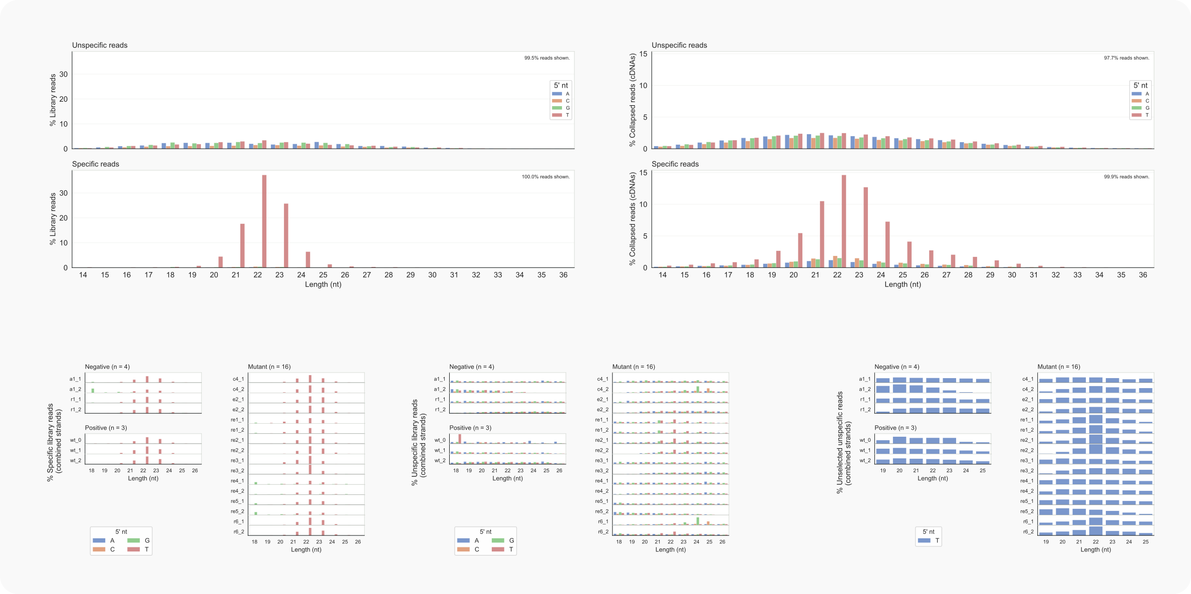
Figure 9. C. neoformans length distributions of library reads.
-lo 1) and collapsed data (cDNAs; -lo 2) on the right.-ld 1, left), unspecific (-ld 1 -k0, middle) and unspecified reads in unspecific data (-ld 6; right).The distribution of read lengths to a narrow range of 20-24 nt with the majority starting with a T (U in RNA) fits expectations for siRNAs bound to Argonaute proteins in fungi [Dumesic-2013]. Furthermore, the separation of specific reads from unspecific reads seems to be adequate in view of the hugely different length distributions for these categories of reads. That putative siRNAs are still present among the unspecific reads in the rde1Δ, rde2Δ or rrp6Δ strains (re1, re2, or r6, bottom middle) appears to be supported by length-distributions for these unselected reads (bottom right) and observations for the rDNA region described below (see Region-analysis).
Multimappers
Transposons that elicit an RNAi response are often present in multiple copies, although some loci might be more active than others, possibly depending on an accumulation of mutations. Therefore, it is not obvious how to account for such repeats during mapping. In the alignment scripts, STAR was set up to map uncollapsed multimappers randomly to the possible loci, while collapsed reads are aligned with each possible position (to keep these hits visible in the bedgraphs) but counted as 1/NH (with NH the number of hits found in the bam alignment line).
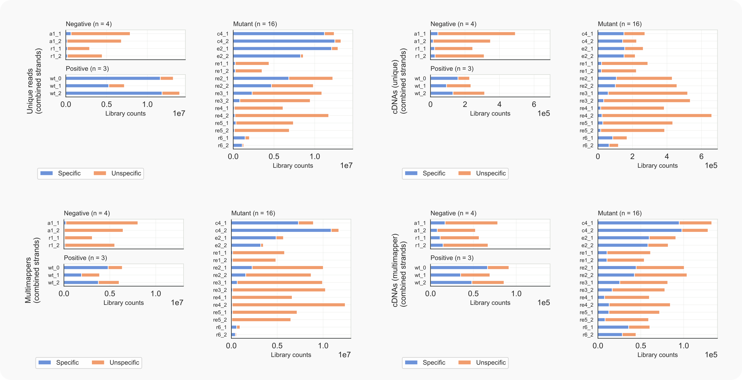
Figure 10. C. neoformans library counts, specific vs. unspecific reads, with focus on unique reads and multimappers.
-lc 1 -ma 1, left) or unique cDNAs (-lc 2 -ma 1, right).-lc 1 -ma 2, left) or multimapping cDNAs (-lc 2 -ma 2, right).The above figure indicates that most of the reads and cDNAs align to a single site (’unique reads’, top) in the reference genome rather than to multiple loci (‘multimappers’, bottom). Centromeres are normally silenced by packaging of nucleosomes into heterochromatin, which coincides with methylation of H3K9 (lysine 9 in histone H3) by Clr4. When this methyltransferase is absent (Mutants c4), the number of multimappers increases (relative to total and unique populations) compared to wild type (Positive wt). Centromeres in Cryptococcus consist mainly of repetitive sequences derived from retrotransposons Tcn1–Tcn5 (that belong to the Ty3-gypsy family of retroelements) and Tcn6 (like Ty1-copia) [Yadav-2018]. Therefore, the increase of multimappers in the absence of Clr4 fits a scenario whereby centromeric transcripts, the expression of which is no longer suppressed by methylation, are silenced by RNAi instead. Notably, genes on euchromatic regions of the chromosomes to which large numbers of siRNAs align to often share homology with domains found in transposable elements but are not clearly related to Tcn1-6.
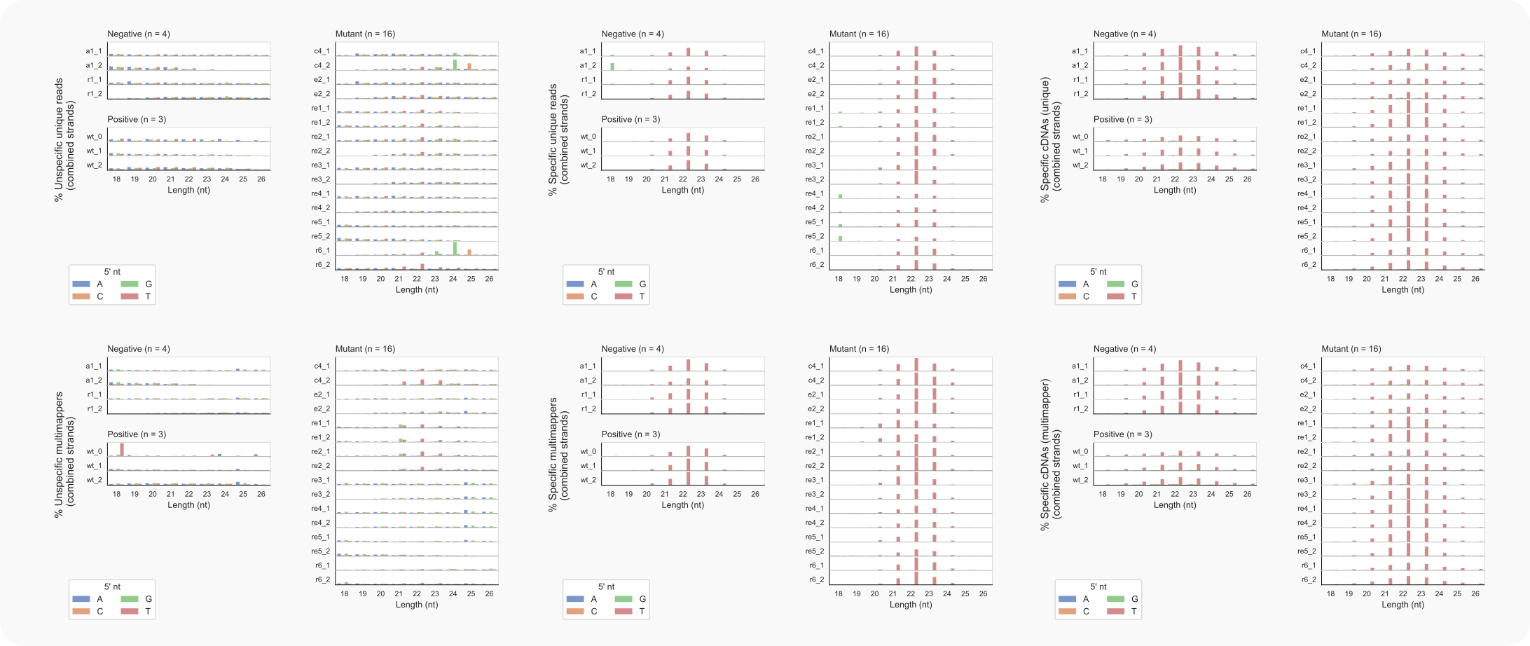
Figure 11. C. neoformans length distributions of unique siRNAs and multimappers.
-ma 1, top) and multimappers (-ma 2, bottom);In the absence of Rde1 only a few siRNAs are found (see Figure 8), defined by cDNAs with a wild-type length distribution (coalispr showcounts -ld 2 -ma {1,2}). Still, most of the multimapping siRNAs (coalispr showcounts -ld 1 -ma 2) in this mutant appear to be 1 nt shorter, peaking with a length of 21 nt, instead of 22 nt (Fig. 11, middle panel, bottom row). Section ‘Multimapping 21-mers in rde1Δ’ tries to find loci responsible for this. One candidate turns out to be the rDNA locus, where such siRNAs map against the pre-rRNA transcript.
Intron-skipping siRNAs
With options -lo {4,5} or -ld {4,5} intron lengths are displayed in uncollapsed reads or collapsed cDNAs, respectively [19]. For a large range of lengths no hits are present. The resolution of the distribution can be enhanced by skipping this empty section. For this:
Edit the field SKIPINT in
3_h99.txt, set it to= 190, 350and save the file.Activate the new configuration by rerunning the
setexp -e h99 -p2command.Redraw the figures.
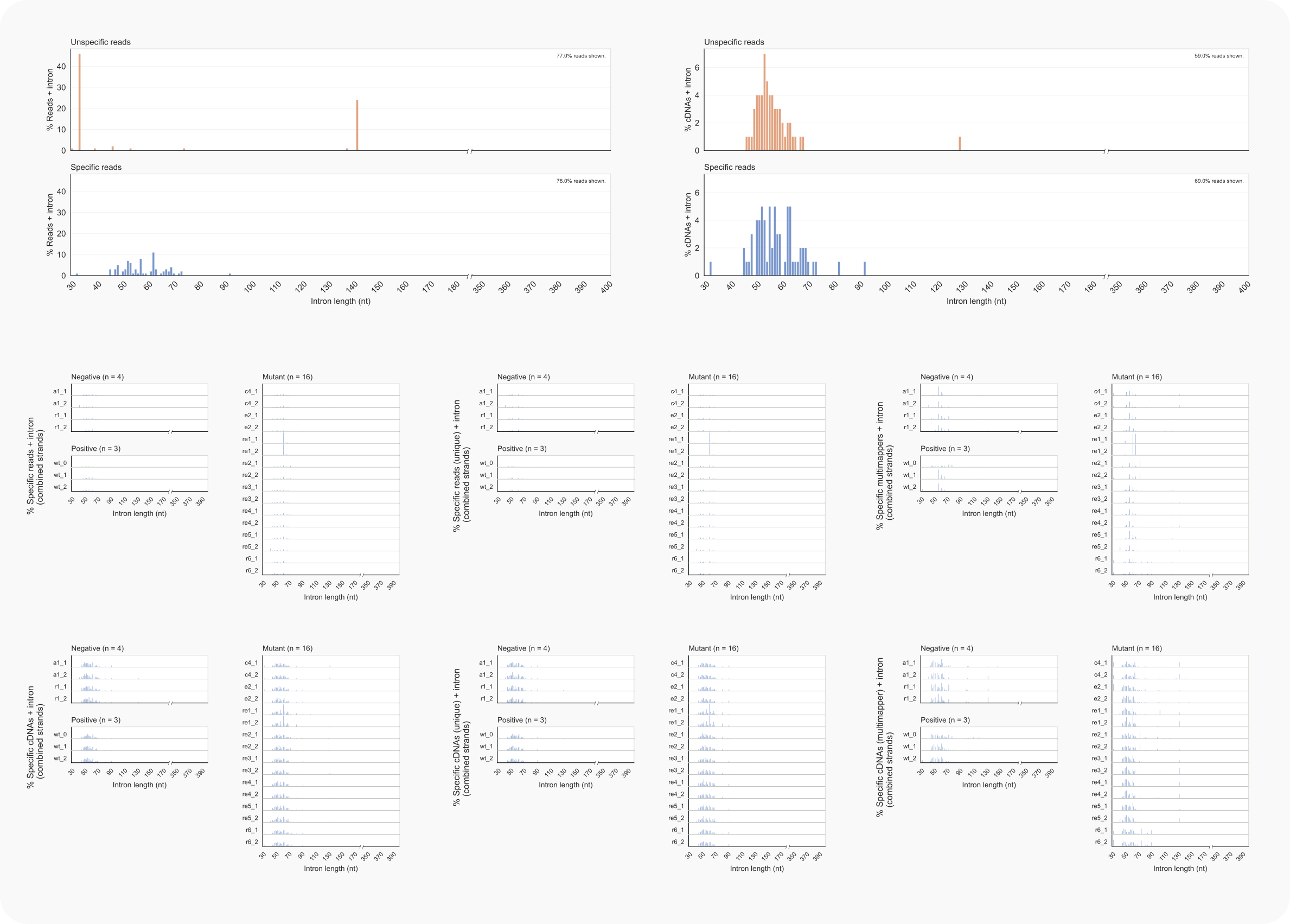
Figure 12. C. neoformans intron lengths of library reads.
-lo 4) and collapsed data (cDNAs; -lo 5) on the right.-ld 4) or cDNAs (Bottom, left -ld 5), unique (middle, -ld {4,5} -ma 1) or multimappers (right, -ld {4,5} -ma 2) for separate libraries.Of the intron-skipping reads, both unique and multimappers bridging an intron of ~62 nt are enriched in the absence of Rde1 (lanes re1 middle section); the number of cDNAs is also relatively increased for these reads, predominantly for those that align to one locus (bottom section, left and middle vs. right panels. In cells without Rde2, multimappers (reads as well as cDNAs) over a spliced intron of ~73 nt stand out (lanes re2 middle and bottom, right). Based on this information, the section ‘Intron-skipping siRNAs’ describes how putative loci can be identified for these reads.
The unique locus from which siRNAs with a 62 nt gap are accumulating in the absence of Rde1 turns out to harbour a unique pseudo-gene, CNAG_07650, on chromosome 6. Centromeric loci account for the multimapper in rde2Δ cells.
Region-analysis
Sometimes, read counts and length-distributions that are valid for just a small section of the overall transcriptome can be highly infomative. Coalispr facilitates this with the coalispr region call. For example, let’s analyze in more detail the rDNA unit in C. neoformans.
rDNA
Obtain images and coordinates for the complete rDNA in H99 from a graph displaying all reads:
Run
coalispr showgraphs -c2 -w2.Use the zoom-tool to select the region covered by the large peak near position 300.000 [16].
Activate mutant traces with comparable traces (
rde1Δ, rde2Δ,rde3Δ, rde4Δ, rde5Δ, methylΔ, orrrp6Δ) and save each image as png.Clicking the x-axis will generate in the terminal the genomic coordinates for the region displayed; e.g.
2 (271985, 279663).Highlight the coordinates (
271985, 279663) and copy these withShift+Ctrl+Cto the clip-board.
Get counts for the rDNA and count-displays by:
In another terminal type ``coalispr region -c 2 -r ``
After option
-r ``, paste the coordinates copied above with ``Shift+Ctrl+V.To use all available samples, include option
-s 2.Set up strand-specific analysis by including option
-st.Run
coalispr region -c2 -r 271985, 279663 -s2 -st 2for PLUS reads and associated diagrams.
The terminal will display which samples are counted; the number of skipped reads, a dataframe showing total numbers and feedback for the figures that are made and automatically saved to the indicated folders [21]. The generated count data are saved as separate files in
/<path_to/Burke-2019/Coalispr/data/h99/tsvfiles/region_readcounts_collapsed-bam/region_2_271985-279663[22].Run
coalispr region -c2 -r 271985, 279663 -s2 -st 3for MINUS reads and associated diagrams.
The obtained diagrams have been combined into Figure 13:
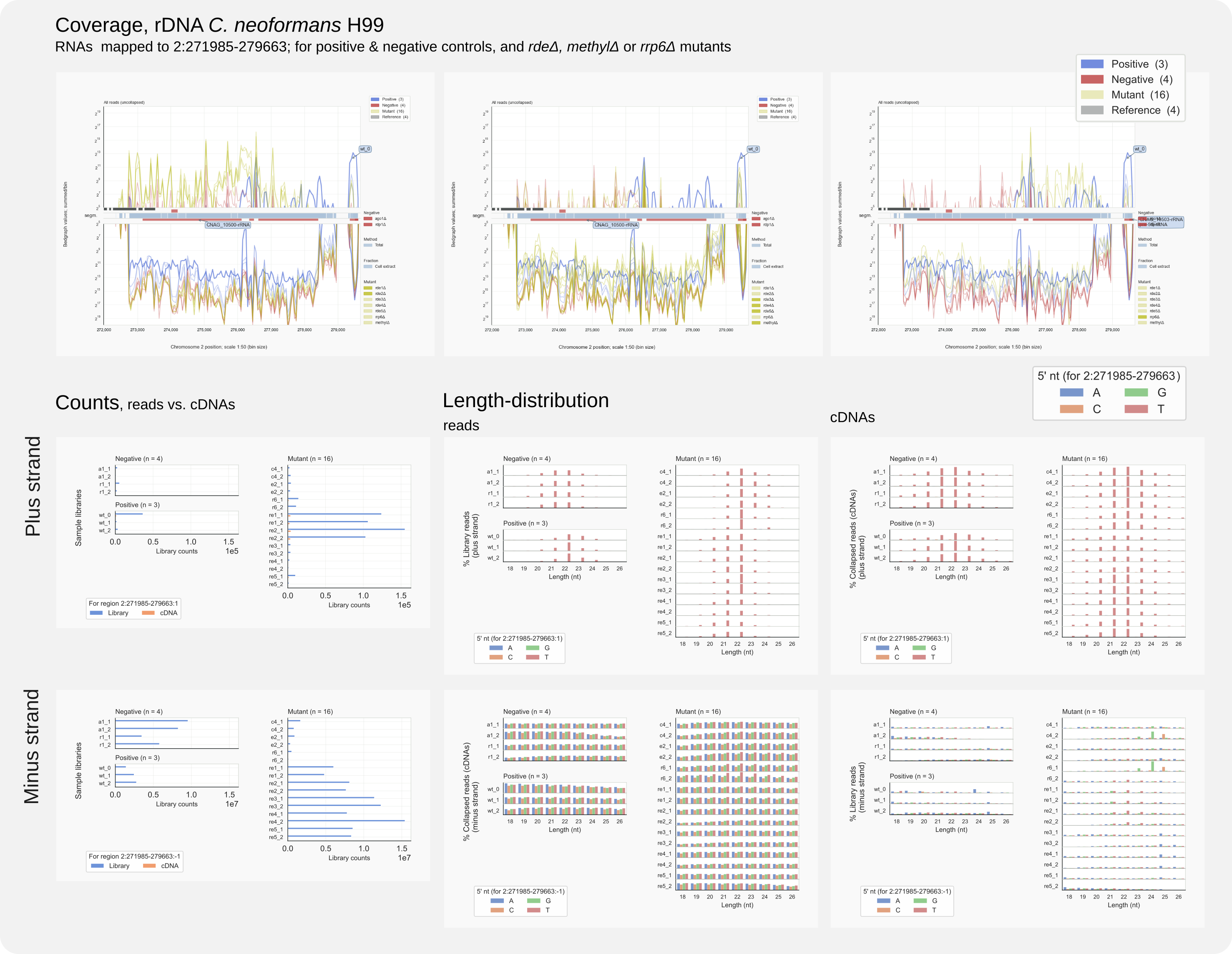
Figure 13. Region analysis of C. neoformans rDNA on chromosome 2.
Various bits of information can be distilled from this figure. When focusing on reads mapping to the rDNA sense strand (minus strand):
RNA fragments formed from ribosomal RNA (the rRFs) are very abundant in negative controls and rde mutants affecting RNAi (
re1tore5) and more so than in strains producing siRNAs (Positive) that could participate in reverse transcription reactions that create the input for the sequencing (see bottom row, left panel).rRFs form the majority of overall unspecific library counts (cf. Fig. 8, top left panel)
The rRFs do not meet the criteria for Ago-associated small RNAs that have a length of 19-23 nt and start with a U (T in cDNA) (see bottom row, middle panel for reads and right panel for cDNAs [23]).
That, despite the high number of counts, rRFS represent uninformative background is illustrated by the coverage pattern of these RNAs, which is the same for all samples (see top panel).
Interestingly, RNAs mapping to the antisense rDNA strand, suggest that siRNAs have been generated against rRNA:
A large number of antisense, plus strand reads were counted for strains rde1Δ (
re1), rde2Δ (re2) and a positive control (wt_0) (Middle row, left panel). See also Fig. 16 (top) below.In all samples, these antisense reads conform to siRNA characteristics.
Different from wild type siRNAs, those in mutant strains appear in general to be 1 nt shorter.
It cannot be ruled out that for samples with low counts these putative siRNAs are an experimental artefact or a kind of background. Still, the high levels of these reads for rde1Δ and rde2Δ strains suggest that in these mutants the RNAi activity could have been redirected to rRNA from transcripts that, somehow, no longer form a target. Thus, a step that would have lead to the generation of specific siRNAs against transcripts from pseudo-genes or transposable-elements is no longer happening because of these mutations.
21-mers
Are the siRNAs only shorter for the rDNA locus in strains rde1Δ or rde2Δ? We can check this for CNAG_07650, one of the few loci with siRNAs in the absence of Rde1 (see Figure 12). The coverage graphs in the section ‘Intron-skipping siRNAs’ show that the major target is the transcript from this pseudo-gene on the plus strand. After zooming the display to only show the region with siRNA traces, obtain the coordinates (say 1371800-1372650) by clicking the x-axis and copy-paste the numbers to run:
Run
coalispr region -c6 -r 1371800-1372650 -s2 -st {2,3}
The combined output indicates that at this locus siRNAs are not shorther in mutant cells, compared to wild type:
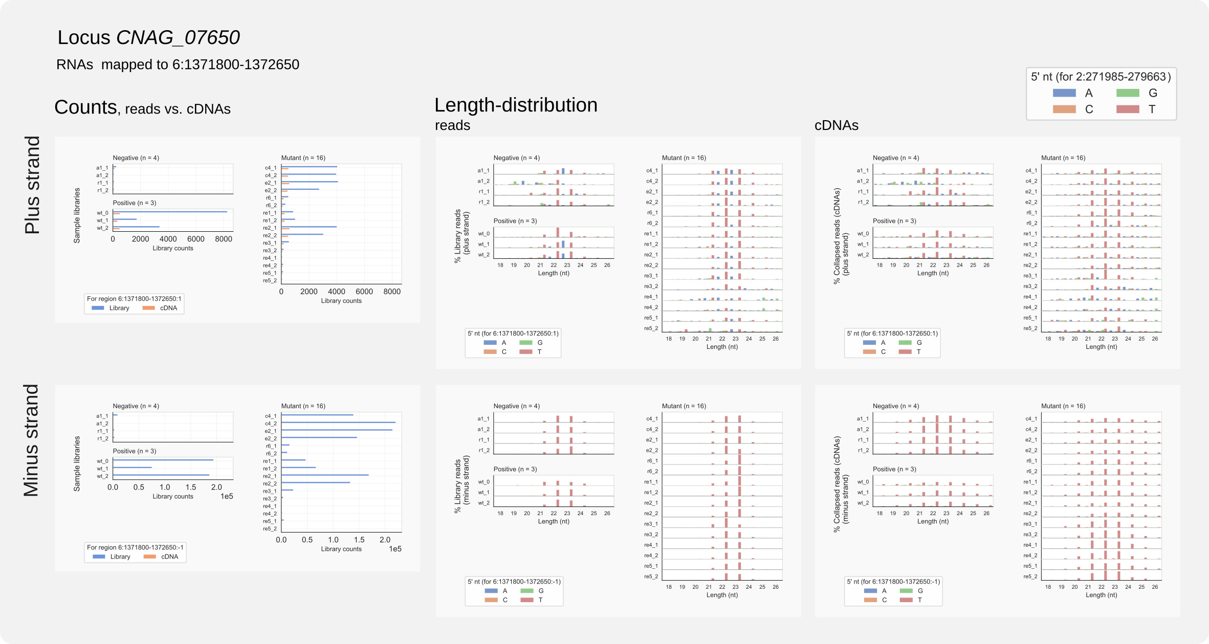
Figure 14. Region analysis of C. neoformans CNAG_07650 on chromosome 6.
CNAG_07650 sequences are not repeated in the H99 genome and this outcome fits the length-distribution for unique loci (Fig. 11, middle panel, top row).
For rde1Δ cells a multimapper was responsible for relative accumulation of siRNAs of 21 nt (see Fig. 11 middle panel, bottom row). This quick analysis suggest that shortening of siRNAs could be linked to the rDNA locus.
Note that for strains with inactivated RNAi (ago1Δ or rdp1Δ), RNAs are still mapping to the CNAG_07650 locus with siRNA length-distributions. For other RNAi loci such background is observed as well. Whether incomplete RNAi-inactivation or library contamination could be the reason for this, is unclear.
auto-RNAi
Above analysis for the rDNA showed that in some strains siRNAs are detected that are antisense to rRFs (Fig. 13). Are other common ncRNAs prone to be targeted by RNAi? It looks that this can happen in the case of SRP RNA as well, another prominent source of unspecific reads. SRP RNA gets expressed from the minus strand on chromosome 1 and is part of a cytoplasmic RNP that associates with ribosomes to regulate translation of proteins that localize to the ER.
Run
coalispr showgraphs -c1 -r 801150-801450 -w2for the coverage display.Run
coalispr region -c1 -r 801150-801450 -s2 -st {2,3}for the count diagrams.
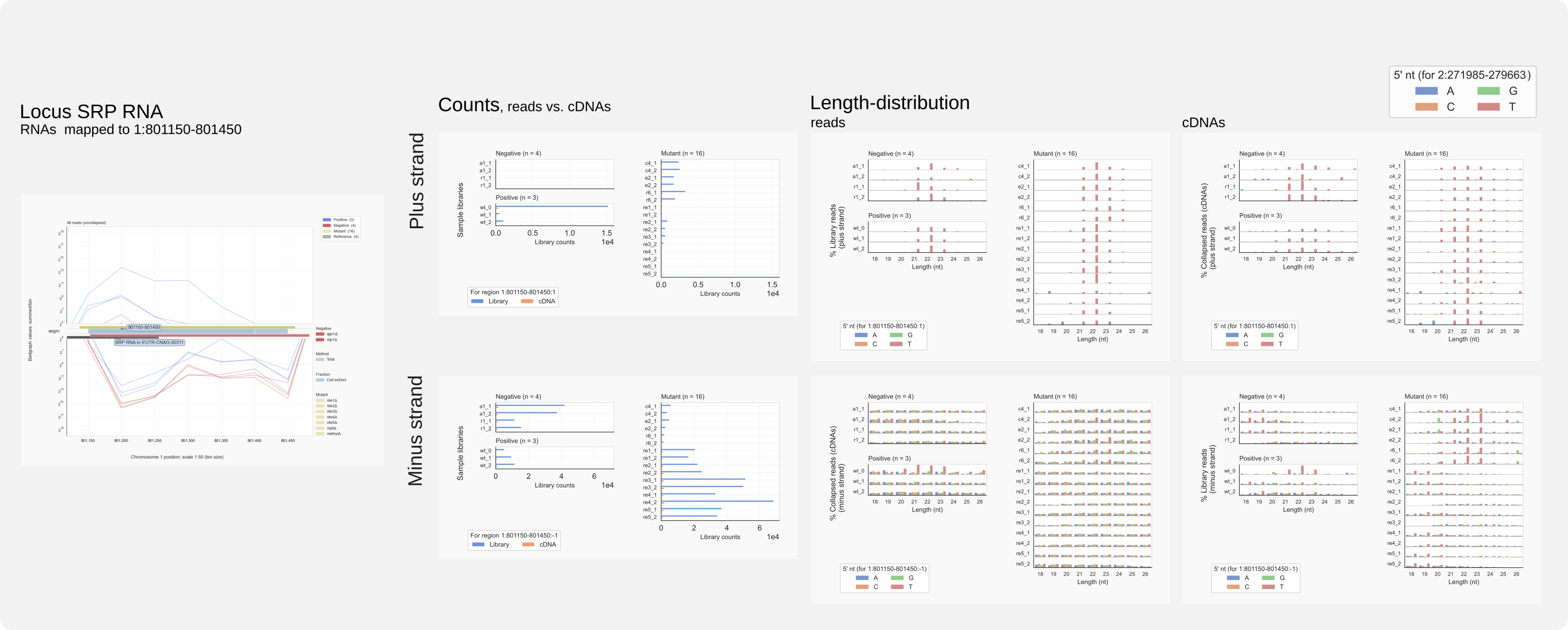
Figure 15. Region analysis of C. neoformans SRP RNA locus.
Note that, for this unspecific locus in RNAi capable strains, cDNAs are found representing CORB sense siRNAs and the more abundant MUNR antisense siRNAs. In strains where RNAi has been affected, the cDNAs for CORB cDNAs do not adhere to a siRNA length-distribution. At loci with specific reads, such reads were observed in low amounts for strains where RNAi had been inactivated (for example CNAG_07650). Such ‘background’(?) signals may have been too low at unspecific loci to stand out as siRNAs in these strains.
If these siRNAs against ncRNAs are really formed, these siRNAs show activity against molecules representing ‘self’, like a sort of auto-immune response but then for RNAi, ‘auto-RNAi’. This also occurs in C. deneoformans, against similar ncRNAs (rRNA, SRP RNA). Such events might indicate that processes involving these ncRNAs triggered RNAi. A common factor is translation. [26]
Annotate count files
The available reference files with genome annotations can be scanned for overlap with segments to which siRNAs map. For this run the coalispr annotate command. Include the mRNA references with -rf 1 an, to easier assess large count numbers, take their log2 values:
coalispr annotate -lg 1 -rf 1
And for unspecific reads (-k0):
coalispr annotate -lg 1 -rf 1 -k0
To get counts for unspecific reads opposite rRNA sequences, include the CORB strand option (-st 3):
coalispr annotate -lg 1 -rf 1 -k0 -st 3
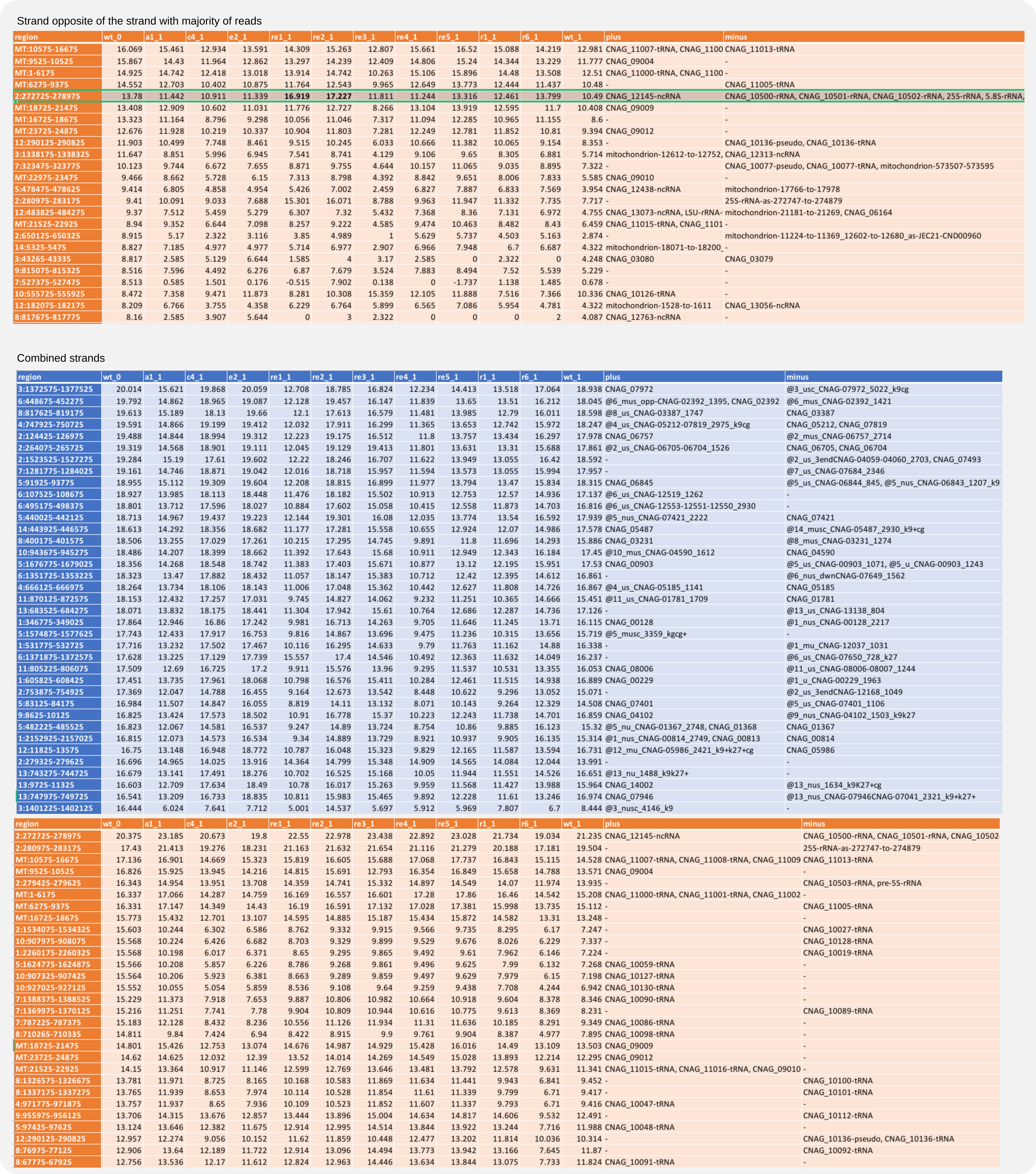
Figure 16. Annotated counts (log2 values).
As found for mouse, in these small RNA-Seq libraries for C. neoformans the counts for rRFs are among the highest read numbers. Most unspecific reads relate to rRNA, tRNA and mitochondrial transcripts; most specific reads are opposite uncharacterized genes.
Conclusion
In the analysis of siRNAs and unspecific RNAs for various libraries prepared by [Dumesic-2013] and [Burke-2019] many observations were linked to rde1Δ and rde2Δ. RDE1 (CNAG_01848) codes for a G-patch protein similar to Sqs1/Pfa1 in Saccharomyces cerevisiae, one of the cofactors for Prp43. This multi-functional RNA helicase relies on G-patch proteins for functional specificity [Bohnsack-2022, Karika-2026]. In yeast, the Prp43/Sqs1 complex is linked to the last step in the maturation of 18S rRNA, cytoplasmic cleavage of 20S pre-rRNA [Lebaron-2009, Pertschy-2009]. In association with alternative G-patch proteins (CMG1, NTR1, Pxr1), Prp43 is further involved in dissociation of spliceosomes and the removal of snoRNPs responsible for 2’-O methylation of 18S and 25S rRNA [Bohnsack-2009, Karika-2026].
Other RNA-processing factors were identified by Burke et al., namely the RNAse III Rnt1 (CNAG_06643, or RDE3), which, in yeast, is a nuclear protein (for a review see [Elela-2018]) and involved in co-transcriptional pre-rRNA processing, analogous to bacterial RNAse III [Abou Elela-1996], and maturation of snoRNAs such as U14 [Chanfreau-1998a, Chanfreau-1998b]. Overall, 13% of the yeast genes are differentially overexpressed in rnt1Δ cells. Yeast Rnt1 carries a characteristic C-terminal RNA-binding domain (RBM0) not present in homologous proteins in fungi that harbour an RNAi machinery. Cryptococcus Rnt1/Rde3 lacks this domain [25] and therefore might not be constrained to double strand RNA substrates formed by NGNN stemloops recognized by RBM0 as is the case for yeast Rnt1 [Elela-2018]. Rde5 (CNAG_04791), with no known orthologues, appeared to be a Rnt1-interacting protein [Burke-2019]. Rde2 (CNAG_04954) is placed among the orthologues of human EDC4, an enhancer of mRNA decapping enzymes, while Rde4 (CNAG_01157) contains domains that suggest it is an orthologue of the TENT5 family of terminal nucleotidyltransferases involved in polyadenylation during 3’ end processing of RNA and linked to the regulation of the innate immune response in animals [Warkocki-2018, Liudkovska-2022].

Figure 17. RNAi onset occurs after splicing.
Disruption of these factors activated the Harbinger transposon to jump from the context of a URA5 reporter gene, and resulted in reduced siRNA production. Because such deletions can be expected to primarily affect ribosome synthesis or mRNA degradation, it cannot be ruled out that a subdued RNAi response could be an indirect result of these deletions. Information from experiments that assess splicing, RNA turnover, and maturation of pre-rRNA and ribosomal subunits in rdeΔ strains will be needed to understand what is actually happening in these cells.
Either way, in rdeΔ strains an RNAi response would be alleviated when this process is triggered by stalled ribosomes and thus directed to ‘difficult’ mRNAs that cause this (Fig. 17). After ribosomes have stalled, a quality control mechanism involving mRNA degradation is initiated by decapping enzymes and 3’ end processing. A lack of sufficient numbers of ribosomes might reduce their chance of collapsing into each other and thereby the onset of clearing processes that also involve RNAi and the generation of siRNAs.
The model cannot explain how siRNAs are maintained and propagated during cell division if the relevant transcripts are not synthesized [24]. That translation might provide a relevant context for the onset of RNAi in Cryptococcus is indicated by the fact that many siRNAs mapped to pseudo-genes and TE-loci, but not - in C. deneoformans - to T1 [Janbon-2010], an active, non-coding transposable element [van.Nues-202?]. Recently it has been found that in stem cells of planarians (a kind of flatworm) piRNA generation is associated with the pioneer round of translation, directly involving the argonaute-like PIWI protein SMEDWI-1 [Parambil-2023]. Thus, route 1 in the model, priming RNAi on problematic transcripts, might occur during such a pioneer round or through common translation on cytoplasmic ribosomes [27]. Another hint in the case of Cryptococcus might be given by the amounts of siRNAs that map anti-sense to mature rRNA (Figure 13), or SRP RNA (Figure 15), in rde1Δ strains and in repair strains where RNAi has been re-established by restoration of genes for Ago1 or Rdp1 [van.Nues-202?]. Maybe such RNAs are mistakenly turned into targets when stalled translation complexes are resolved. Would this also mean that cells need to “learn” that some RNAs, like rRNA, are self?