Mouse miRNAs

Data accumulated by [Sarshad-2018] on mouse Argonaute-miRNA complexes had been used in a bioinformatics meta-analysis that claimed that ribosomal RNA (rRNAs) fragments (rRFs) were a novel class of small RNAs that bind to Argonaute.

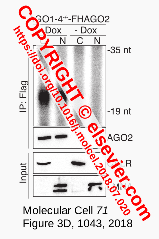
Figure 1. Input RNA

Sarshad-2018, Figure 3D];

© cell.com; elsevier.com.

RNA depicted in the + Dox lanes of Figure 3D in [Sarshad-2018] (Fig. 1) was equivalent to the input for high throughput sequencing that yielded one of the datasets used to support that claim.

Experience with RNA-seq in yeast and fungi (see About) where rRNA and tRNA were common contaminants inspired development of Coalispr. This tutorial uses the program to assess whether rRFs belong to specific or unspecific reads in the mouse miRNA datasets of [Sarshad-2018]. Neiher rRFs nor the - Dox miRNA-Seq datasets were explicitly discussed in this publication, although the analysis of experimental results will have involved comparison to negative data. For controls, the meta-analysis referred to Figure 3D,F as claim for a clean input, raising the question whether unspecific fragments had been taken into account that could have been amplified significantly during subsequent PCR steps of library preparation and sequencing. This opens up the possibility that rRF-signals correspond to the background smear shared with the negative control (lanes - Dox) rather than the miRNAs in the well-defined band of ~22 nt (Fig. 1). In other words, it cannot be excluded that the binding of rRFs to AGO2 as suggested by the meta-analysis was not specific and represented an experimental artefact.

Dataset

The data for [Sarshad-2018] had been deposited at GEO under number GSE108801, with GSE108799 as accession number for the miRNA data corresponding to Fig. 1. Accession number GSE108799, however, yielded 12 libraries with 50 nt sequences with little overlap to the set of identified miRNAs. Thankfully, the authors sent the miRNA dataset used for the paper (which consists of 8 libraries, see Fig. 2) after an email communication. At the time of writing, these datasets - which were kindly provided by M. Hafner - were not (yet?) accessible via the primary Geo accession number.

Note

Outcome of below data-preparation can be downloaded from xenodo.org. See/skip to here

Set up the work environment for this tutorial:

• create a work directory to store data, scripts and other files; name it, say Sarshad-2018/.

• copy the contents of this folder in the source distribution: coalispr/docs/_source/tutorials/Mouse/shared/ to Sarshad-2018/.

• open a terminal and run cd \<path to>\Sarshad-2018 to run below scripts in this, the expected, work environment.

SRA accession numbers for each data set are listed in SRR_Acc_List.txt, originally obtained via GEO for GSE108799. Correspondence with the received data files is described in the GSE108799_ExpTable.tab configuration file (see below )

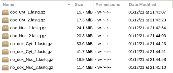
Figure 2. miRNA seq data [Sarshad-2018]

Like for the yeast, or H99 tutorials, to obtain the raw data from GEO one can use the SRA-Toolkit and then run scripts to retrieve the data sets [1]. When files are directly requested from the authors (and assuming they will ship the same data set as used here), create the following directory structure:

• for Coalispr scripts to work, each of the SRR6442834-44 names will need to be represented as subfolder/dataset within the Sarshad-2018/ working directory:

Sarshad-2018
├── SRR6442834
│   └── SRR6442834.fastq.gz (symbolic link to/renamed "dox_Nuc_1.fastq.gz")
├── ..
├── SRR6442844
│   └── SRR6442844.fastq.gz (symbolic link to/renamed "no_dox_Cyt_2.fastq.gz")

• in each SRR6442834-44 subfolder, create a symbolic link with name SRR6442833(-44).fastq.gz to the corresponding compressed data file; alternatively, place (a copy of) the data file into the subfolder and rename it accordingly.

Alignment

Before the data can be aligned with STAR to the mouse genome, we have to obtain reference files. Following the paper, we get most files from Gencode (see source-references.txt).

Genome

Obtain a fasta file for the genome:

• wget http://ftp.ebi.ac.uk/pub/databases/gencode/Gencode_mouse/release_M30/GRCm39.genome.fa.gz

STAR needs unzipped fasta for reading the sequence; run:

• gunzip -k GRCm39.genome.fa.gz

Create a link to a fasta file that is not version-specific. This is used in all scripts, and makes it easier when an updated version is used. Run:

• ln -s GRCm39.genome.fa GRCm.genome.fa

We are mainly interested in rRNA fragments (rRFs). Therefore we ignore introns and generate a genome index (required by STAR) without a reference file. The script needs a name for the folder, which will be based on EXP, as the first argument (i.e. ‘mouse’). With the DNA file as second argument run:

• 1_1-star-indices.sh mouse GRCm.genome.fa

  (script with input parameter fasta file GRCm.genome.fa)

  This will take some time and uses up a lot of RAM. After this step is complete, the computer might still be sluggish. Maybe because shared memory is not cleared. [2]

Mapping

The data that was transferred by dropbox were pre-trimmed with Cutadapt but need to be cleared from empty reads that block STAR. Therefore:

• copy python script coalispr/coalispr/resources/share/no_empty_fa.py to Sarshad-2018/, then run:

• sh 2_1-collapse-pre-trimmed-seqs.sh

  (to obtain collapsed read files with pyFastqDuplicateRemover.py from pyCRAC and remove the empty read),

• sh 2_2-clean-uncollapsed-pre-trimmed-seqs.sh

  (to clear uncollapsed read files from empty reads).

The reads can now be aligned. Loading the reference genome for mapping takes a lot of time for the first alignment; it needs about ~25 Gb of free RAM [2]. The alignment scripts are set up to load the genome and then keep it in shared memory, which works fine on a single computer. When the mapping is done on a cluster of shared computers, this can cause problems (see STAR/issues/604); edit the bash scripts 3_1 and 4_1 so that the setting NoSharedMemory is activated.

Alignments and subsequent files will be stored in two directories within Sashad-2018 that will be created by the scripts, namely STAR-analysis0-mouse_collapsed/ and STAR-analysis0-mouse_uncollapsed/. The folder names contain the EXP parameter (i.e. ‘mouse’) which is the first argument for the mapping scripts. To align the collapsed reads with zero mismatches [3] :

• sh 3_1-run-star-collapsed-14mer.sh mouse

Do the same for the uncollapsed reads, run:

• sh 4_1-run-star-uncollapsed-14mer.sh mouse

  Remove the genome from shared memory (if that is used) when all mapping threads (set to 4 in the script) have completely finished:

• sh 4_1_2-remove-genome-from-shared-memory.sh mouse

And create bedgraphs for both collapsed and uncollapsed data sets by [3]:

• sh 3_2-run-make-bedgraphs.sh mouse

• sh 4_2-run-make-bedgraphs-uncollapsed.sh mouse

Note that the alignments are stored in their own subdirectories and that the filenames (Aligned.out.bam, Log.final.out etc.) are the same for each experiment. Therefore, Coalispr uses the folder names as a lead for retrieving bedgraph and bam files.

If Fastqc and RSeQC are installed, some quality control of the alignments can be done. Still, most relevant information (concerning the percentage of mapped reads) is already provided in the log files generated by STAR. So it is optional to run sh 5_1-QC-reports.sh mouse [3]. Still, fastqc gives a quick overview of sequence characteristics and can highlight frequent sequences in uncollapsed fastq data or in unmapped reads. This is handy for checking common contaminants or sequences that could not be mapped due to mismatches, as shown in this table.

References

For using Coalispr a tabbed file with the lengths of the chromosomes is required; its name is set as field LENGTHSNAM in the configuration. When STAR has been used for mapping, this file is available, namely chrNameLength.txt in the star-mouse folder (created by script 1_0-star-indices.sh). To make it easily accessible make a short-cut to this file and run:

• ln -s star-mouse/chrNameLength.txt GRCm_genome_fa-chrlengths.tsv [4]

Annotations for various kinds of RNA will be helpful and can be retrieved from a general GTF (see source-references.txt), which can be obtained by:

• wget http://ftp.ebi.ac.uk/pub/databases/gencode/Gencode_mouse/release_M30/gencode.vM30.chr_patch_hapl_scaff.annotation.gtf.gz

  To reduce alterations to scripts etc. when updated versions of the annotation file becomes available, create a link mouse_annotation.gtf.gz which is used as the reference here:

• ln -s gencode.vM30.chr_patch_hapl_scaff.annotation.gtf.gz mouse_annotation.gtf.gz

The mouse annotation contains information for common ncRNAs that could be expected as contaminants [5] (like tRNA, snRNA, snoRNA and rRNA). A negative-control reference file common_ncRNAs.gtf (used as GTFUNSPNAM in the program settings) is built as follows:

• copy python script coalispr/coalispr/resources/share/sub_gtf.py to Sarshad-2018/, then run:

• sh 6_1-common-ncRNAs.sh [7]

An annotation file for a positive control would describe small RNAs expected to bind to AGO2, like miRNAs (sense overlap), or their targets (anti-sense overlap). We extract miRNA sequences from the annotation [6] and predicted targets after retrieving these from miRDB [Chen-2020]. Download targets by:

• wget http://mirdb.org/download/miRDB_v6.0_prediction_result.txt.gz

  To facilitate use of other versions, a link (miRDB.gz) to this source file will be used as input for the scripts below:

• ln -s miRDB_v6.0_prediction_result.txt.gz miRDB.gz

  The positions for the miRNAs and their potential targets are extracted from the general annotation file (downloaded above). To find the target information a correct gene-id is needed, for which the file gene2ensembl.gz comes in handy:

• wget https://ftp.ncbi.nlm.nih.gov/gene/DATA/gene2ensembl.gz.

The following steps will gather miRNA sequence annotations [8] into the file miRNAs.gtf (used for setting GTFSPECNAM) and their targets into miRNAtargets.gtf (field GTFREFNAM):

• copy python script coalispr/coalispr/resources/share/get_smallRNAs_and_targets.py to Sarshad-2018/, then run:

• sh 6_2-collect-miRNAs-and-targets.sh [9]

If other information (from another gtf or gff file) needs to be combined with these files, this should be possible [10].

Note

Datasets prepared above were uploaded to xenodo.org (DOI 10.5281/zenodo.12822543). These can also be used for testing Coalispr.

• cd <path to workfolder>

• wget -cNrnd --show-progress --timestamping "https://zenodo.org/records/12822544/files/Sarshad-2018.tar.gz?download=1"

• tar -xvzf Sarshad-2018.tar.gz

Coalispr

Setup

For Coalispr to function properly, a work environment needs to be prepared and associated with the program during set up.

Work folder

After above preparation of the input data, which can also be downloaded from zeonodo.org, processing by Coalispr can begin. First a reference name and work environment for the program will be created. The work folder can be set up in the user’s home/ folder, in the current folder or within the distribution folder. Here, we will keep the distribution and files in the home folder separate from the output from Coalispr. Instead, we will place the output near the input data and create a Coalispr/ folder within Sashad-2018/.

As before, in a terminal change directory to your work environment by:

• cd /<path to>/Sarshad-2018/

init

All conditions are met to initiate Coalispr. For that, in the context of the work-environment, run:

• coalispr init

  and:

• give the session a name, say mouse and confirm. This sets the reference EXP for this experiment.

• choose the current folder (option 2) as destination and confirm.

  On the terminal the following output is shown:

Configuration files to edit are in:
'/<path to>/Sarshad-2018/Coalispr/config/constant_in'
The path '/<path to>/Sarshad-2018/Coalispr' will be set as 'SAVEIN' in 3_mouse.txt.

At this stage the bare requirements for using Coalispr as described in the how-to guides have been initialized. This step also generates output (sub)folders in the Coalispr folder. The next and major requirement is to complete two files, one describing the experiment (EXPFILE) and the other, the configuration file (3_EXP.txt) with settings for the program concerning data, the EXPFILE, GTF annotation files etc.

Configuration

In the ‘How-to guides’ it is explained that Coalispr relies on two kind of files that configure the program. One file, the EXPFILE describes the experiment, while constants and other settings are put in 2_shared.txt and 3_EXP.txt that get combined to build the constant.py source file used by all scripts (modules). Below is described how the EXPFILE and configuration files are created.

Note

When using the archive with alignments downloaded from xenodo.org, the EXPFILE GSE108799_Exp.tsv and configuration files are present. You only need to edit the shipped configuration file /<path to>/Sarshad-2018/Coalispr/constant_in/3_mouse_zenodo.txt:

• From 3_mouse.txt created by coalispr init, copy relevant [12] values for:

  • SETBASE

  • SAVEIN (BASEDIR / PRGNAM).

  and replace those in 3_mouse_zenodo.txt

• Remove/rename 3_mouse.txt

• Rename/link 3_mouse_zenodo.txt to 3_mouse.txt

Experiment file

As a basis for the EXPFILE, one could use the SraRunTable.txt found with the SRA data files using the link on GEO. This is a csv file and a tsv format is required.

In line with the Experiment file section of the how-to guides we will add columns covering a SHORT name (with “A2” for AGO2, “n” for nuclear and “t” for total), and CATEGORY. Here, via file XtraColumns.txt, we also provide experimental descriptions (“Exp_Name”) found on the GEO site and names of the data-files received per dropbox. The “Run” column gives SRA accession numbers. These form automatically the names of folders when downloading data from GEO with the SRA-Toolkit. Therefore, the SRR names can be directly used as links to the unique bam and bedgraph files in the subfolders. For this reason, “Run” from SraRunTable.txt is by default the header of the FILEKEY column with keys for merging the files. Of the other columns of interest, METHOD and FRACTION, the latter is present in SraRunTable.txt. Another required column, CONDITION, is empty because the two conditions of induction (with or without doxycyclin) have already been accounted for in defining the negative and positive controls in CATEGORY.

Run           Fraction  Exp_Name           PerDropBox     Short   Category  Group   Method      Condition
SRR6442834    Nuc       ESC_Nuc_dox_1      dox_Nuc_1      A2n_1   S         A2n     rip2
SRR6442835    Nuc       ESC_Nuc_dox_2      dox_Nuc_2      A2n_2   S         A2n     rip2
SRR6442837    Nuc       ESC_Nuc_nodox_1    no_dox_Nuc_1   n_1     U         n       rip2
SRR6442838    Nuc       ESC_Nuc_nodox_2    no_dox_Nuc_1   n_2     U         n       rip2
SRR6442840    Total     ESC_Total_dox_1    dox_Cyt_1      A2t_1   S         A2t     rip2
SRR6442841    Total     ESC_Total_dox_2    dox_Cyt_2      A2t_2   S         A2t     rip2
SRR6442843    Total     ESC_Total_nodox_1  no_dox_Cyt_1   t_1     U         t       rip2
SRR6442844    Total     ESC_Total_nodox_2  no_dox_Cyt_2   t_2     U         t       rip2

The following steps accomplish this:

• copy python script coalispr/coalispr/resources/share/cols_from_csv_to_tab.py to Sarshad-2018/, then run:

• python3 cols_from_csv_to_tab.py -f SraRunTable.txt -t 1 -e XtraColumns.txt

  (-f is input file, -t 1 stands for “tutorial 1”, the one for Mouse miRNAs; -e for “expand with”)

The results are written to file GSE108799_Exp.tsv (similar to GSE108799_ExpTable.tab).

Settings file

The second file to prepare is a copy of the 3_EXP.txt configuration file, namely 3_mouse.txt. This file was prepared by coalispr init and contain all settings needed for Coalispr to function properly with the mouse data. The file to edit is in Coalispr/config/constant_in within Sarshad-2018/ (see above output of coalispr init), which can be checked using command ls; by running:

• ls Coalispr/config/constant_in

Edit Coalispr/config/constant_in/3_mouse.txt, with a text editor like scite, run:

• scite Coalispr/config/constant_in/3_mouse.txt

  (by setting Language in the menu-bar to “Python” the active fields are highlighted compared to the comments)

All lines beginning with ‘#’ will be ignored when this file is processed. Fields that can be set are NNNNN = a setting while #NNNNN indicates an alternative but unused setting. Removing the ‘#’ at the start of this line will activate this field. Some fields in this file have been already been set: EXP refers to “mouse”, and the SAVEIN storage folder. The field SRCFLDR will result by default in names beginning with “STAR-analysis0-mouse_” [11] for folders with bedgraphs and bam alignments with 0 mismatches for EXP.

Fields to be altered in the template (‘#’ indicates a comment):

• EXP : “mouse” [12]

• CONFNAM : “3_mouse.txt” [12]

• EXPNAM : “Mus musculus”

• LOG2BG : 4

• USEGAPS : BINSTEP [13]

• MIRNAPKBUF : 1/5 [14]

• CNTRS : [CNTREAD, CNTCDNA, CNTSKIP]

• LENCNTRS : [LENREAD, LENCDNA]

• MMAPCNTRS : [ [LIBR] ]

• CHROMLBL : “” [15]

• SETBASE : “/<path to>/Sarshad-2018/”

• EXPFILNAM : “GSE108799_Exp.tsv”

• CYTO : “Total”

• EXPERIMENT : “Exp_Name”

• MUTGROUPS{

  “n” : “nuclear nodox”,

  “t” : “cytoplasmic nodox”,

  “A2n” : “AGO2 ip, nuclear”,

  “A2t” : “AGO2 ip, cytoplasmic”,

  }

• UNSPECIFICS : [ “n”, “t”, ]

• MUTANTS : “”

• LENGTHSNAM : “GRCm_genome_fa-chrlengths.tsv”

• GTFSPECNAM : “miRNAs.gtf” [16]

• GTFUNSPNAM : “common_ncRNAs.gtf” [17]

• GTFREFNAM : “miRNAtargets.gtf” [18]

• SAVEIN : Path(“/<path to>/Sarshad-2018/Coalispr”) [12]

• LENGTHSFILE : BASEDIR / LENGTHSNAM [19] [20]

• EXPFILE : BASEDIR / EXPFILNAM

• GTFSPEC : BASEDIR / GTFSPECNAM

• GTFUNSP : BASEDIR / GTFUNSPNAM

• GTFREF : BASEDIR / GTFREFNAM

Test, reset

After saving the 3_mouse.txt file, we have to test that Coalispr can work with the new configuration. Run from within the Sarshad-2018/ work directory:

• coalispr setexp -e mouse -p2

  (option -e indicates EXP and -p2 to choose a path to a configuration file; see coalispr setexp -h)

Choose option 2 and confirm. If all python formatting is fine, the process terminates with:

Configuration '/<path to>coalispr/coalispr/resources/constant.py' ready for experiment 'mouse'

Typos, however, can easily be made, or adjusting the wrong field. Such errors only show up at the next run (when the program relies on the configuration for start-up). Therefore, to check that the configuration is correct, one can repeat the last command coalispr setexp -e mouse -p2 or run, for example, the help menu coalispr -h.

If that happens to fail, or the repeat appears different from the first run, some setting is wrong. The working order of Coalispr can be restored by resetting the configuration via python3 -m coalispr.resources.constant_in.make_constant. It is possible to compare a version of the configuration that worked at authors’ end [21] and shipped with the program (check-3_mouse.txt) with the prepared one using gvim: gvimdiff check-3_mouse.txt Coalispr/config/constant_in/3_mouse.txt [22].

Analysis

After preparing the configuration files, the bedgraphs prepared from the alignments can be processed.

setexp

First, we have to set Coalispr to use the mouse configuration (stored in the work-environment); run:

• cd /<path to>/Sarshad-2018/

• coalispr setexp -e mouse -p2

  choose option 2 and confirm.

storedata

The next step is to convert the bedgraph data into Pandas dataframes, saved as pickle files by Coalispr. The storedata command is used for this, the options for which can be checked with:

• coalispr storedata -h

Note

When using the archive with alignments downloaded from xenodo.org, this step can be skipped and binary, processed data that is used in Coalispr can be obtained with coalispr storedata -d4 after which subsequent commands (like coalispr showgraphs or coalispr countbams) can be tested. After this, or when generating your own data files through coalispr storedata -d{1,2} -t{1,2} remove or rename the backup_from_pickled link (to prevent that the contents shipped with the archive are overwritten by subsequent coalispr storedata -d3 commands).

No reference bedgraphs will be used [23]. First, store the data for the uncollapsed reads (the default type, -t1):

• coalispr storedata -d1

  The output on the terminal:

Bedgraphs of 'uncollapsed' and aligned reads for experiment 'mouse' are now collected and processed.

Processing bedgraphs ...

Binned bedgraph-frames are being created for 'A2t_2'; this will take some time
Binned bedgraph-frames are being created for 'n_1'; this will take some time
Binned bedgraph-frames are being created for 'A2n_1'; this will take some time
Binned bedgraph-frames are being created for 't_1'; this will take some time
Binned bedgraph-frames are being created for 'A2t_1'; this will take some time
Binned bedgraph-frames are being created for 'A2n_2'; this will take some time
Binned bedgraph-frames are being created for 't_2'; this will take some time
Binned bedgraph-frames are being created for 'n_2'; this will take some time
bin_bedgraphs for plus-strand A2t_2
Processing input file '/<path-to>/Sarshad-2018/STAR-analysis_uncollapsed/SRR6442841_uncollapsed_1mismatch/SRR6442841_uncollapsed_1mismatch-plus.bedgraph'
..

Run the same command including option -t2 to store the data for collapsed reads:

• coalispr storedata -d1 -t2

During these steps, various scripts are run, one of which merges the data and split this in categories of specific and unspecific reads. This speciation depends on some settings, like UNSPECLOG10 (see: How-to guides).

info

With coalispr info options -r1 and then -r2 or -r3 the effect of various parameters on the number of specified regions can be visualized (this takes a while).

Figure 3. Contiguous regions for uncollapsed data by coalispr info -r2 [24]

The default UNSPECLOG10 setting of 0.905 requires a minimal difference of ~8-fold between read signals in positive controls and those in negative controls to mark the former as specific; a smaller difference will specify the reads forming the peak as unspecific. Mostly, however, positive control samples will introduce signals that are absent from the negative control.

Errors could occur [25]. Apart from terminal output, info that can help find the origin of such an error can be found in the logs [26].

coalispr showgraphs -c chr17 -w2

Figure 4. rRNA reads are not specific to AGO2, while those for expressed miRNAs are.

showgraphs

The bedgraph traces of the stored data can now been displayed with coalispr showgraphs. Let us look at the ribosomal RNA genes in the mouse genome:

The sequences coding for ribosomal RNAs are present as rDNA repeating units. A 45S rRNA, which serves as the precursor for the 18S, 5.8S and 28S rRNA, is transcribed from each rDNA unit by RNA polymerase I. The number of rDNA repeating units varies between individuals and from chromosome to chromosome, although usually 30 to 40 repeats are found on each chromosome.

—from Rn18s

Of these rDNA repeats, an 18S unit on chromosome 17 [27] is annotated for the reference genome. Either use the zoom tools or visualize the 18S region using option -r1:

• coalispr showgraphs -c chr17 -r1

• a dialog is presented to give the coordinates:

• provide the range [27] plus some flanking sequence:

  (40152000, 40161000), confirm.

The top panel of Fig. 4 shows traces for nuclear (and cytoplasmic) negative controls that are indistinguishable from those for the AGO2 IPs. Compare this to loci for miRNA genes, expected to be covered by reads associated with AGO2 rather than those isolated from the un-induced samples. This can be seen in the range (18050000, 18052000) on chromosome 17: there is an miRNA cluster of Mir99b, Mirlet7e, and Mir125a (while ENSMUSG0000207560 was not detected). Based on these observations rRFs cannot be proven to be specifically associated with AGO2 in this data-set.

countbams

The alignment files can be counted in various ways. For total inputs, run the next command twice, once with option -rc 1 for uncollapsed reads and then with -rc 2 for collapsed data:

• coalispr countbams -rc {1,2}

  (these counts can be checked with showcounts -rc)

The specified reads that have been aligned can be counted in two runs as well. For specific reads use the command:

• coalispr countbams

With option -k 2, the unspecific reads are counted:

• coalispr countbams -k2

showcounts

If input totals have been counted with countbams -rc {1,2}, these can be displayed with:

• coalispr showcounts -rc {1,2}

with this outcome:

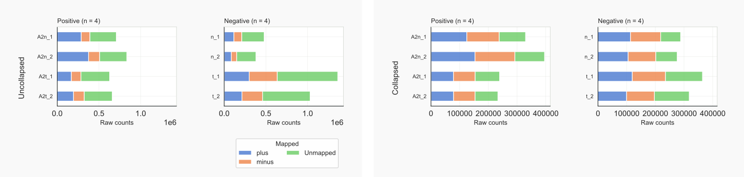
Figure 5. Input counts by coalispr showcounts -rc {1,2} [28]

Collapsed input shows that complexity of the libraries are comparable. About 1/3 of cytoplasmic cDNAs (t_1, t_2 , right panel) were not mapped, although these formed a large section of the data-set before collapsing (left panel). Many reads of the negative controls mapped to repeated loci. In contrast, AGO2-associated RNAs appear to align mostly to unique genomic sequences. Less than 1% of reads were not counted based on an imperfect alignment according to the cigar string. This can be seen by comparing uniq and total library counts and by comparing the number of reads that were skipped with total library counts, all visualized with:

• coalispr showcounts -lc {1,2,9}

Figure 6. Library counts by coalispr showcounts -lc {1,2,9}

Numbers are shown for uniq (-lc 2, left), all (-lc 1, mid) and skipped (-lc 9, right) reads.

Note that a large portion of reads in the induced (positive control) samples are not associated with AGO2 but overlap with those in the uninduced, negative controls (and therefore referred to as unspecific). The rRFs, at least those derived from 18S rRNA (Fig 4), belong to this class; such reads also do not share characteristics of specific reads only found with AGO2.

Most reads associated with AGO2 have a defined length restricted to 21-23 nt and begin with an A. The unspecific reads common to all samples, however, are enriched around 31-33 nt and begin with a G. This is shown by the overview on the left, obtained with option -lo 1 in:

• coalispr showcounts -lo 1 |-ld 1 -k {1,2}

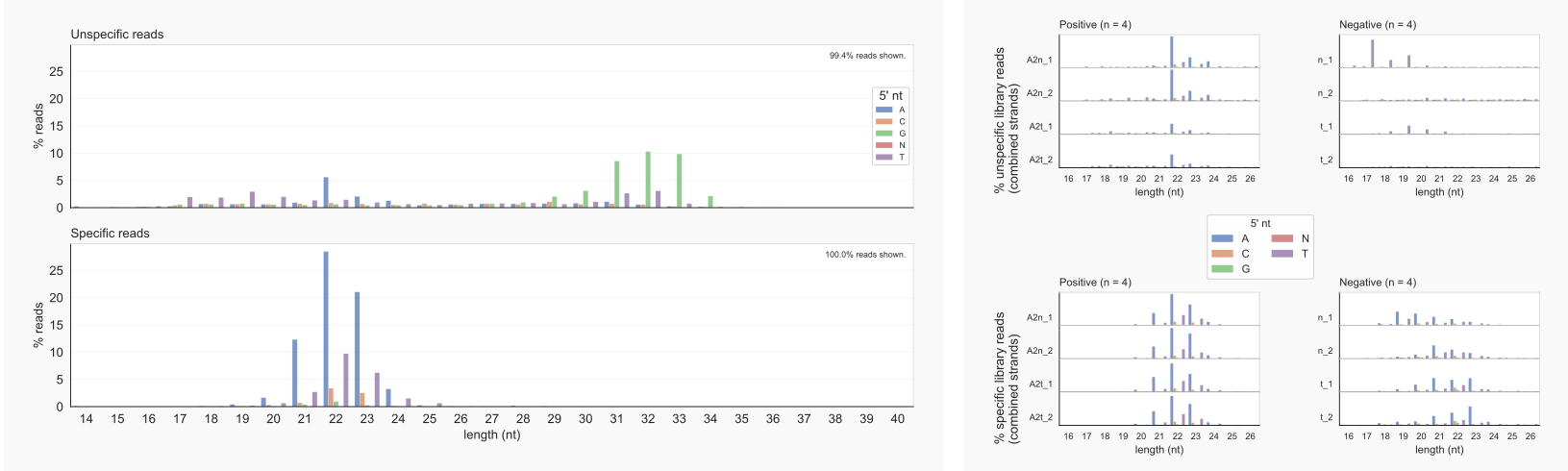
Figure 7. Read-length distributions by coalispr showcounts -lo 1 | -ld 1 -k {1,2} [29]

In the right panel, reads for separate libraries of the positive controls (‘Specific’) and negative controls (‘Unspecific’) are classified; the upper panels show length-distributions for reads that were specified as unspecific (options -ld 1 -k2). Reads that were counted in regions that were standing out as specific (option -ld 1 (-k1)) are in the lower panels. Reads were found in negative controls that map to genomic segments with more than 10^UNSPECLOG10-fold signal in the positive controls. These ‘specific reads’ in unspecific samples, however, appear to have a different distribution than those linked to AGO2 (bottom right, right panel). Also, false negatives are apparent: 22-mers starting with an A in AGO2 nuclear samples (top left, right panel), were present in regions with mostly unspecific reads. This could happen when unspecific and specific reads form different peaks, that, however, are too close together to occupy different bins. It is also possible that the reads overlap but that a difference in peak height did not meet the set threshold for declaring them to be specific.

Below the same has been done for cDNAs (i.e. collapsed reads), still indicating an AGO2-specific length distribution. Assuming that the 5’ nt does not affect adapter ligation or PCR amplification during the library preparation, more identical RNA molecules with an A at the 5’ end, especially those with a length of 22 and 23 nt, would have been present in the input sample. The abundant cDNAs with a T as 5’ nt do not represent as many reads at those beginning with an A.

• coalispr showcounts -lo 4 |-ld 4 -k {1,2}

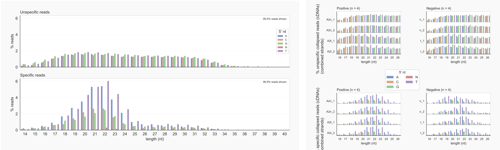
Figure 8. cDNA-length distributions by coalispr showcounts -lo 4 | -ld 4 -k {1,2} [29]

The peak of unspecific reads with a G as 5’ nt and a length of about 32 nt is no longer visible after collapsing. These reads do not appear to derive from the rDNA unit (see below).

Include 45S pre-rRNA

For an analysis with Coalispr, extra DNA can be added on top of the official annotations. This can be useful when (portions of) genes have been introduced into the cells that are not part of the genome of the organism under study. Think of inducible promoters, epitopes, selectable markers, or guide sequences that may end up in the transcriptome but cannot be mapped by lack of a reference. Fairly common too, is that the assembly of the reference genome (still) misses particular, but known features. For example, the mouse genome lacks a complete rDNA unit that encodes the 45S pre-ribosomal RNA from which the mature 18S small subunit rRNA and the large subunit rRNAs, 5.8S and 28S, are derived [30]. Above, we have only shown reads aligned to the 18S portion of the rDNA unit; here we will add the 45S containing sequence from accession no. X82564 to check whether the large subunit 28S and 5.8S rRNAs attract many reads [31].

This requires editing the settings in the configuration file.

Initiate the new experiment in the work directory Sarshad-2018:

• coalispr init

• Let’s name the experiment ‘mouse45s’.

For the configuration, maybe easiest is to make a copy of the existing 3_mouse.txt and replace the 3_mouse45s.txt created by coalispr init by:

• cp 3_mouse.txt 3_mouse45s.txt

Then edit the following fields in 3_mouse45s.txt to use the extra DNA [31] and save.

• EXP : “mouse45s”

• CONFNAM : “3_mouse45s.txt”

• BAMSTART : “A” [32]

• LENGTHSNAM : “GRCm_genome_fa-45s-chrlengths.tsv”

• LENXTRA : 22118

• DNAXTRNAM : “mmu-45S_ENA-X82564.fa”

• DNAXTRA : BASEDIR / DNAXTRNAM [19] [20]

• CHRXTRA : “mmu-45S_ENA-X82564”

• GTFUNXTNAM : “Rn45s.gtf”

• GTFUNXTR : BASEDIR / GTFUNXTNAM

Note

When using the alignments downloaded from xenodo.org, edit shipped configuration file /<path to>/Sarshad-2018/Coalispr/constant_in/3_mouse45s_zenodo.txt:

• From 3_mouse45s.txt created by coalispr init, copy relevant [12] values for:

  • SAVEIN (BASEDIR / PRGNAM).

  • SETBASE

  and replace those in 3_mouse45s_zenodo.txt

• Remove/rename 3_mouse45s.txt

• Rename/link 3_mouse45s_zenodo.txt to 3_mouse45s.txt

coalispr showgraphs -c mmu-46S_ENA-X82564 -w2.

Figure 9. Sequenced rRNA fragments (rRFs) are not specific to AGO2.

All (top), nuclear (2^nd) and cytoplasmic (3^rd and bottom) rRF signals. The only positive control signal exceeding that of negative control samples is in the 18S and not reproducible (bottom).

The fields GTFXTRANAM and GTFXTRA are not used here, because the added rDNA belongs to the common non-coding RNA (defined by GTFUNSP). For this, a new annotation dataframe is build by Coalispr from the previously made common_ncRNAs.gtf (from GTFUNSP) and Rn45s.gtf (from GTFUNXTR), put together by comparing alignments of various precursor and mature rRNA molecules [31].

We have to re-align the reads to the now expanded mouse genome, for which we have to make novel indices. STAR allows for extra fasta input during genome generation; just include the two fasta files that form the ‘mouse45s’ genome during this step:

• sh 1_1-star-indices.sh mouse45s GRCm.genome.fa mmu-45S_ENA-X82564.fa

  This will take quite a while

Make a link to the novel genome-lengths file:

• ln -s star-mouse45s/chrNameLength.txt  GRCm_genome_fa-45s-chrlengths.tsv

Then do the remapping; alignments and derived bedgraphs are stored in a new set of folders created by the scriptrs linking them to EXP (‘mouse45s’) [11]:

• sh 3_1-run-star-collapsed-14mer.sh mouse45s [3]

The same for the uncollapsed reads:

• sh 4_1-run-star-uncollapsed-14mer.sh mouse45s

Clear the RAM:

• sh 4_1_2-remove-genome-from-shared-memory.sh mouse45s

Create the bedgraphs:

• sh 3_2-run-make-bedgraphs.sh mouse45s

• sh 4_2-run-make-bedgraphs-uncollapsed.sh mouse45s

Process the bedgraphs with Coalispr:

• coalispr setexp -e mouse45s -p2

• coalispr storedata -d1

• coalispr storedata -d1 -t2

  (Sorry, these data collection steps take a very long time.)

coalispr showgraphs -c mmu-45S_ENA-X82564 -w2 -t2 -u1

Figure 10. Unselected rRF-cDNAs.

Comparable miRNA-like cDNA’s (orange) map to mature regions of 45S (top) like 28S (bottom) for all samples.

Check traces:

• coalispr showgraphs -c chr17 -w2

• coalispr showgraphs -c mmu-45S_ENA-X82564 -w2

Gather counts:

• coalispr countbams -rc 1

  for input uncollapsed reads.

• coalispr countbams -rc 2

  for input collapsed reads.

• coalispr countbams

  for mapped specific reads.

• coalispr countbams -k2 -u1

  for unspecific reads (-k2), also save (-wb 1)

  and count ones that fit the miRNA pattern (-u).

Check traces for missed miRNA-like cDNAs (Fig. 10) in collapsed data:

• coalispr showgraphs -c mmu-45S_ENA-X82564 -w2 -t2 -u1

  (-t2 for collapsed data, because from these the unselected reads `u1 are gathered during the counting.)

Compare input counts for data mapped to the mouse genome, as above (Fig. 5), and after inclusion of the 45S rDNA (Fig. 11):

• coalispr showcounts -rc 1

• coalispr showcounts -rc 2

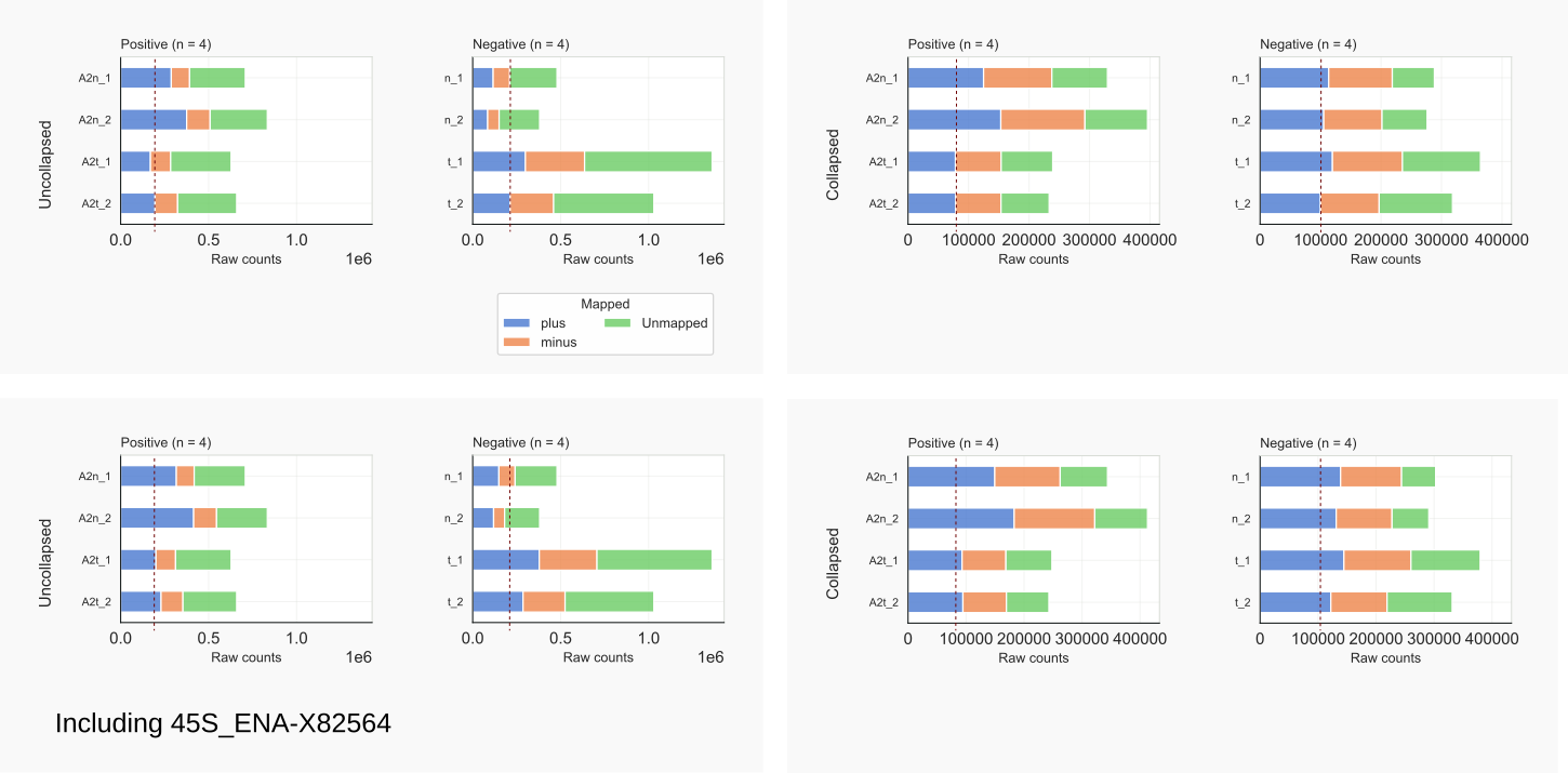
Figure 11. Input counts by coalispr showcounts -rc {1,2} [28]

Data for the reference mouse genome (top), including 45S rDNA (bottom).

Including the 45S rDNA has enlarged the numbers of reads (Fig. 11 bottom left) and cDNAs (bottom right) mapping to the PLUS strand (blue) as could be expected [31]. The bars representing the unmapped reads (green) have become shorter accordingly. No big changes are observed when comparing overall library counts obtained with:

• coalispr showcounts -lc {1,2,9}

Figure 12. Library counts by coalispr showcounts -lc {1,2,9}

Comparison of mapped reads before (top) and after inclusion of 45S rDNA (bottom).

Uniq (-lc 2, left), all (-lc 1, mid) and skipped (-lc 9, right) reads.

After addition of the 45S rDNA to the genome, more unspecific cDNAs are mapped (Fig. 12 left), but overall counts did not change by much in general. Slightly less reads appear to be classified as specific; maybe because some of these actually map to the 45S rDNA. The distribution of read - or cDNA lengths (Figs. 13, 14) did not change either, compared to the analysis above without 45S rDNA mapping (Fig. 7):

• coalispr showcounts -lo {1,4} |-ld {1,4} -k {1,2}

Figure 13. Read-length distributions by coalispr showcounts -lo 1 | -ld 1 -k {1,2} [29]

Figure 14. cDNA-length distributions by coalispr showcounts -lo 4 | -ld 4 -k {1,2} [29]

Figure 15. cDNA-lengths by coalispr showcounts -ld 8

Overall, adding the 45S rDNA does not affect the major observations concerning the specific reads associated with AGO2 that derive from miRNAs. The typical length distribution, from 16 to 25 nt peaking at 22 nt, is also not found in the group of unspecific reads that fit the length and 5’ nt characteristics of miRNAs (Fig. 15); a singular 22 nt peak is seen among specific reads that flattens in the negative control with:

• coalispr showcounts -ld 8

region

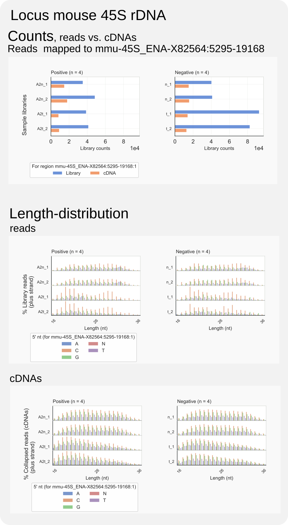
Figure 16. Mouse rRF-cDNAs and rRFs.

No specific enrichment of a class

of rRFs in positive samples on the

basis of counts (top) or length-

distributions in comparison to the

negative controls.

The command coalispr region -c B -r <region>, which specially analyses reads for a particular genomic region (<region>) on a chromosome B, can help to get a more precise idea of the kind of reads and cDNAs that map to the 45S rDNA on the positive strand. The following command will yield overal counts and length distributions of these rRFs:

• coalispr region -c mmu-45S_ENA-X82564 -r 5295-19168 -st 2

The command, as explained in the How-to guides, creates and saves the diagrams of Fig. 16. The counts in the top panel indicate most rRFs derive from rRNA in the cytosol of the negative control, and these have C as the preferable 5’ nt (middle panel). Still, their lenght distributions do not significantly differ from those for AGO2-associated rRFs (middle panel), also in the case of cDNAs (bottom panel).

Among the total of unspecific reads, a peak of RNAs of around 32 nt in length that started with a G was observed (Fig. 7), also when including the complete rDNA (Fig. 13 ). These reads do not appear to consist of rRFs; the region-analysis in Fig. 16 shows that such peak was absent in the fraction of reads mapping to the 45S rDNA.

annotate

The obtained count files can be checked against available reference files with coalispr annotate, which helps to illustrate the outcomes and the working of the program in another way. Below figure (Fig. 17) shows the results of coalispr annotate. The command selects available reference files dependent on the kind of read (-k). To get tables after scanning all GTF annotations, that is including those for a REFERENCE (represented by GTFREFNAM; pointing to a file with miRNA targets), use option -rf 1 as done in the following commands. For the specific reads, which automatically scans GTFSPECNAM (file miRNAs.gtf), run:

• coalispr annotate -rf 1

For the unspecific reads, that are always compared to the negative-control reference file, GTFUNSPNAM (common_ncRNAs.gtf), set option -k as well:

• coalispr annotate -rf 1 -k2

Inclusion of a general reference GTF can extend processing time so that it can take a while to generate the output in the form of .tsv files that are saved in Sarshad-2018/Coalispr/outputs/mouse45s/. The data will be sorted so that the most abundant reads will be at the top (to turn sorting off, include option -sv 0). Adding option -lg 2 will provide the log2 values of the counts. For pretty printing of the table, the output files can be formatted after loading these in a program like WPS Office.

The table for unspecific reads shows that rRFs are among the most abundant counted reads in the dataset (Fig. 17 bottom left, row 1). Significant numbers of specific and unspecific reads derive from the same genomic regions expressing miRNA clusters but relate to different sections as shown in the trace diagrams on the right.

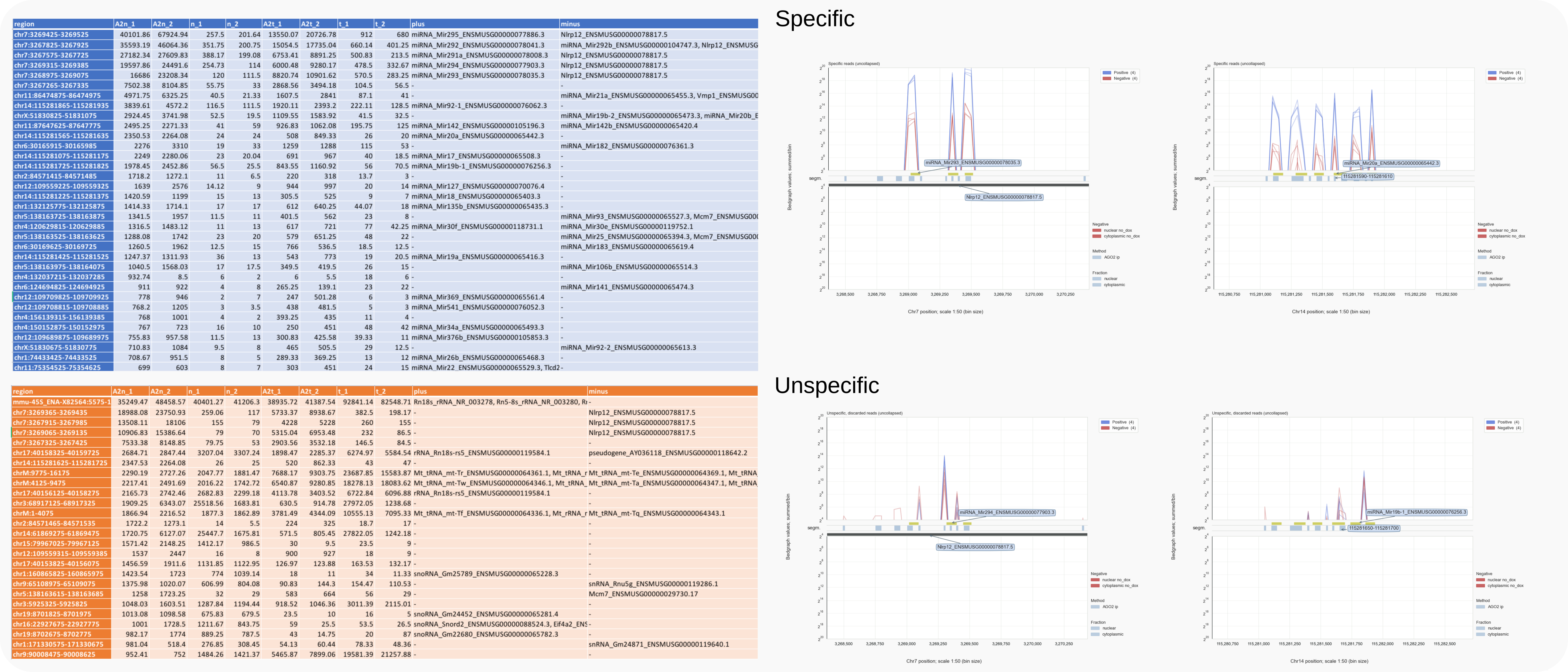
Figure 17. Mouse count data annotated and compared to traces for miRNA clusters on chromosomes 7 or 14.

Top section of the tables (left) obtained with coalispr annotate -rf 1 for specific reads (top) and unspecific reads (-k 2, bottom) compared to diagrams obtained with coalispr showgraphs -c chr7 -r 3268365-3270435 or coalispr showgraphs -c  chr14 -r 115280625-115282725 (right). The tables have been formatted after loading the .tsv output files in WPS Office.

A particular selection can be obtained by using various options. To obtain a list of cDNAs for reads that map to unique genomic positions (-ma 1), this command could be used:

• coalispr annotate -lc 2 -ma 1

Compare this to the table with all specific cDNAs obtained with

• coalispr annotate -lc 2

The reduced numbers of unique cDNAs (Fig. 18 left panel) shows that some in the total number of cDNAs (Fig. 18 right panel) have been mapped to several genomic positions. Also note the relative small difference between cDNA numbers for positive control samples (A2..) and negative controls (n_.., t_..), while these difference can be enormous in the case of library read numbers above (Fig. 17). This suggests that multiple, identical cDNAs could have been made from multiple reads of the same sequence and length, that is from identical miRNAs, exceeding vastly in number those present in the negative controls.

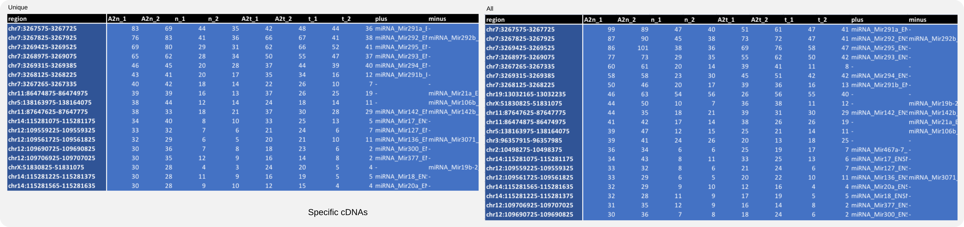
Figure 18. Annotated mouse count data for specific cDNAs.

Gene descriptions and count numbers for unique cDNAs (left) and for the total cDNA library (right). Multimappers account for numerical differences [33].

Thus, with coalispr annotate a comparison between counts and known genes can be added after counting of the specified reads with coalispr countbams, which is done independently of the annotations and is solely based on the genomic regions identified to be covered by reads that confer information concerning the biological system under study, here miRNAs binding to AGO2 in mouse.

Conclusion

Overall, the outcomes of this analysis can not support that rRFs associate with mouse AGO2 in a biologically meaningful manner. Possibly, this idea originated from bioinformatics analysis not incorporating available negative control data.

• Mouse-shared
• Commonly unmapped

---

Notes

[1]

If still present, remove adapters by means of Flexbar or, as done by the authors, with Cutadapt.

[2] (1,2)

The terminal can appear locked up, especially after interruption of any of the previous STAR commands (that is when they did not complete properly). On the terminal or in the STAR Log.out messages can provide a hint. If a line mentions that STAR is halting because of a genome in shared memory, then: stop the currently running STAR and release the blockage by running sh 4_1_2-remove-genome-from-shared-memory.sh from the terminal from within the working directory with the genome reference folder. At the authors end this worked, but some errors have ben seen [STAR feedback]. Scripts have been adapted to bypass these errors, but if RAM is still occupied after trying to clear it; try closing the terminal you were working in.

[3] (1,2,3,4,5)

Add the number of allowed mismatches in the alignment as the second argument for the script: sh 3_1-run-star-collapsed-14mer.sh mouse 1 for 1 mismatch with the mouse genome. When mapping is redone with the same number of mismatches existent alignment folders within SRCFLDR [11] will be renamed from SRR644.. to _SRR644..

[4]

Alternatively, if STAR has not been used, one can create this file by running sh 6_0-genomelength.sh GRCm.genome.fa. This uses the script pyCalculateChromosomeLengths.py from pyCRAC and cleans out a repeated part of the fasta headers using shell-commands cut and paste. The resulting file will also be: GRCm_genome_fa-chrlengths.tsv.

[5]

To stress the experiential background of this, the expectation that rRNA fragments are background is based on the observation - shown below - that most signals for rRFs are indistinguishable between sequencing samples. See also the section . It does not exclude the possibility that some rRFs can be found as specifically bound to proteins. This is illustrated in the tutorials for yeast, where data are discussed for processing factors involved in the maturation of pre-rRNA and assembly of ribosomeal sub units. Furthermore, the GTFs annotating common non-coding or other RNAs are not used for counting, only for providing quick feedback when the data is analyzed; they are based on what is known from the literature or public reference databases.

[6]

The miRNA sequences from mirbase [Kozomara-2019] could be an additional resource but these were based on another version of the mouse genome and therefore not used here.

[7]

This is basically the command python3 sub_gtf.py -k common_ncRNAs -a 0 -g mouse_annotation.gtf.gz -f snRNA,snoRNA,tRNA,miscGm;rRNA,misc7SK;scaRNA,miscSRP;Y_RNA;pseudogene; the bash script just defines the input parameters; -a is an option to gather all annotations (1) or the minimal necessary (0) for Coalispr.

[8]

Note that only gtf-features (that is values in column #3) GTFEXON and GTFFEAT are taken into account by Coalispr.

[9]

The bash script calls a python script and sets the input parameters for it: -k (kind) miRNA, -a (all) 0, -t (target-file) miRDB.gz, -g (reference gtf) mouse_annotation.gtf.gz and -o (output) miRNAtargets.gtf while creation of miRNAs.gtf is linked to -k.

[10]

If other files need to be combined with the created outputs, say when a relevant mmu.gff3 becomes available at mirbase you could try to do this. First, download these miRNA sequences: wget https://www.mirbase.org/ftp/22.1/genomes/mmu.gff3 (22.1 is the [Kozomara-2019] version, which will be different for other, more recent releases) and convert mmu.gff3 to gtf: copy coalispr/coalispr/resources/share/convert_gff3.py to Sharshad-2018/ and run python3 convert_gff3.py -f mmu.gff3. Then, combine the output with the relevant file generated before: sh 6_2-collect-miRNAs-and-targets.sh mmu.gtf miRNAs.gtf. This output can then be set as GTFSPECNAM.

[11] (1,2,3)

This setting is the default. STAR-analysis0-mouse_ forms the beginning of the folder names for storing mapping data. These names end in collapsed or uncollapsed and are created by running mapping scripts 3_1 or 4_1. The ‘mouse’ portion relates to the EXP setting. The digit in the name represents the number of mismatches allowed in alignments of reads to the reference genome. The default in the scripts is zero mismatches but this can be set by adding the number as the second argument to the alignment command [3]. The SRCFLDR setting has to reflect this new number to work with the correct data set.

[12] (1,2,3,4,5)

Done during coalispr init step.

[13]

Set to smallest gap possible (which is given by BINSTEP). Most positive peaks are miRNA hits, so account for small single peaks rather than transcript regions targetted by siRNAS.

[14]

Specific hits displayed by showgraphs see figure indicate that miRNAs appear mostly as single peak hits. These are accounted for by the single coordinate of the one bin they end up in. In order to register these peaks for counting, expand the peak by setting the MIRNAPKBUF so that it gets some countable ‘span’. Even when the resolution is increased by reducing the size of the bins (BINSTEP), some peaks are not picked up without setting the MIRNAPKBUF. Resolution increase slows down proceedings, especially with the mouse genome: a binstep of ~20, makes the datastore step very slow.

[15]

Beginning of the x-axis label in displays by coalispr showgraphs, normally ‘Chromosome’ but here redundant.

[16]

This name is output from script 6_2. GTFSPECNAM represents a lane that shows pre-recorded read-overlaps. That is, overlaps not determined by Coalispr but by either manually scanning traces of mapped reads in a genome browser or when such overlaps have been published.

[17]

This name is output from script 6_1. GTFUNSPNAM represents a lane that shows published genomic loci for classes of ncRNAs; many of these overlap with unspecific peaks, defined by their connection to negative controls.

[18]

This file is generated by script 6_2 and holds annotations for putative miRNA targets, so that their names can be seen with coalispr showgraphs.

[19] (1,2)

No quotes (” “) around the text as this is a reference to pre-defined constants; keep spaces around /.

[20] (1,2)

File is placed next to sequence data folders, within the work-directory Sarshad-2019/.

[21]

In the check-3_mouse.txt, the paths to various files are for the author’s system and will NOT be correct for that of the user.

[22]

Assuming that gvim is available; alternatively vimdiff (also needing vim ) or diff can be used.

[23]

This suits the input option for ‘only data’ (-d1).

[24]

The current, default settings for UNSPECLOG10 and LOG2BG are marked (dashed line).

[25]

Depending on the UNSPECLOG10 value, specific reads are identified or not. When errors are shown during this step, it could be that the chosen settings are too stringent. Instead of by coalispr info, a low setting of UNSPECLOG10, say 0.4, can be checked after editing the configuration file.

• In a terminal:

  • scite /<path to>/Sarshad-2018/Coalispr/config/constant_in/3_mouse.txt &

  • change UNSPECLOG10 to 0.4; save

  • cd /<path to>/Sarshad-2018/

  • coalispr setexp -e mouse -p2

  • coalispr storedata -d1

Terminal output may show that some parts have been skipped when done before; the last lines indicate that the genome positions of reads are stored in separate files, one for specific reads, the other for unspecific data with the new setting.

[26]

Output and other messages are collected in log-files. The most recent messages are stored in /<path-to>/Sarshad-2018/Coalispr/logs/mouse/run-log.txt (<path-to-work_folder>/LOGS/EXP/LOGFILNAM). When the program does not run as expected, info can be found there that might help to resolve problems, especially when this was not sent to std.out (standard out, i.e. displayed on the terminal).

[27] (1,2)

Chromosome 17 (40157244-40159092) shows up as the locus with the 18S region after grep -i 18S mouse_annotation.gtf; no results are obtained when searching for 28S or the precursor 45S. While 5.8S is normally within the 45S pre-rRNA in between 18S and 28S rRNA sequences, it is annotated to be on chromosomes 6 (94803762-94803904) and 18 (73666474-73666621).

[28] (1,2)

Input counts for uncollapsed reads with option -rc 1 on the left and for collapsed reads with -rc 2 on the right.

[29] (1,2,3,4)

Overview of lengths, left (coalispr showcounts -lo 1); and in separate libraries, right (coalispr showcounts -ld 1). Reads specified as specific are in the bottom panels; those that show overlap between negative (Category ‘Unspecific’) and positive (Category ‘specific’) control up to the 10^UNSPECLOG10 threshold (on the right), are called unspecific and shown in the upper panels..

[30]

The table with unmapped sequences describes reads associated with 45S pre-rRNA.

[31] (1,2,3,4)

The mouse 45S pre-rRNA sequence comes from accession no. X82564 and is annotated according to acc. no. NR_046233, which places it on chromosome 17. In the fasta file the same seq_id as in the gtf will be used. Alignments of X82564 yielded the coordinates for Rn18s (NR_003277.3); Rn5-8s (NR_003280.2, J01871.1, K01367.1 and human 5.8S rRNA, NT_167214.1 (112024 to 112180)); and Rn28s (NR_003279.1). All sequence annotations place the 45S-associated rDNA on the PLUS strand.

[32]

Based on our first analysis we can adapt the BAMSTART to ‘A’ in the settings, and check for unselected reads among the unspecific ones as will be done below.

[33]

Total cDNAs contain multimappers, which should be reflected in the numbers being floats; the fractions have been omitted here.

STAR feedback

When clearing up RAM did work:

bash-5.1$ sh 4_1_2-remove-genome-from-shared-memory.sh mouse
        STAR --genomeDir /<path to>/Sarshad-2018/star-mouse --genomeLoad Remove --outSAMtype None
        STAR version: 2.7.10a   compiled: 2022-01-31T21:02:42+00:00 /tmp/SBo/STAR-2.7.10a/source
Sep 20 23:36:23 ..... started STAR run
Sep 20 23:36:23 ..... loading genome
Sep 20 23:36:23 ..... started mapping
Sep 20 23:36:23 ..... finished mapping
Sep 20 23:36:23 ..... finished successfully

When a wrong experiment is passed to STAR, the loaded genome cannot be found, according to this error message:

bash-5.2$ sh 4_1_2-remove-genome-from-shared-memory.sh
        STAR --genomeDir /<path to>/Sarshad-2018/star- --genomeLoad Remove --outSAMtype None
        STAR version: 2.7.10a_alpha_220818   compiled: 2022-09-21T00:09:53+01:00 knotsUL:/tmp/SBo/STAR-2.7.10a_alpha_220818/source
Sep 27 14:33:12 ..... started STAR run
Sep 27 14:33:12 ..... loading genome

EXITING: Did not find the genome in memory, did not remove any genomes from shared memory

When a STAR thread was still active this generated an error message:

bash-5.1$ sh 4_1_2-remove-genome-from-shared-memory.sh mouse
        STAR --genomeDir /<path to>/Sarshad-2018/star-mouse --genomeLoad Remove --outSAMtype None
        STAR version: 2.7.10a   compiled: 2022-01-31T21:02:42+00:00 /tmp/SBo/STAR-2.7.10a/source
Sep 02 01:24:03 ..... started STAR run
Sep 02 01:24:03 ..... loading genome

Shared memory error: 11, errno: Operation not permitted(1)
EXITING because of FATAL ERROR:
There was an issue with the shared memory allocation.
Try running STAR with --genomeLoad NoSharedMemory to avoid using shared memory.
Sep 02 01:24:06 ...... FATAL ERROR, exiting