How-to guides
The input for Coalispr are bedgraph files. Starting point is to get these. For this, adapters and barcoded linkers have to be removed from raw reads which then need to be mapped to a reference genome. For some data sets the mapping will have to take introns into account; i.e. the possibility that reads have been spliced [1]. From the obtained alignments, bedgraph files can be generated [2].
In the tutorials these preparations have been included. As also shown, before mapping reads, these can be collapsed to speed up alignment and, more importantly, the counting of reads. The program selects the sections of the alignment file to count and collapsed reads only need to be counted once to obtain the number of all identical reads present in the library. Together with figures of bedgraph traces, the resultant counts (and linked figures) are the main output of Coalispr.
Here, how Coalispr works is explained; how it can help to clean up the data by means of negative controls. The program prepares counted data, which then can be further analyzed.
Rationale
The overall idea behind this application is that the output of negative biological controls is common to all samples, and relate to the kind of experimental methods used. These negative controls show which part of the experimental output is not informative. Therefore, removing this unspecific output from all samples gives signals that are specific, both for the positive control and for mutant or test samples analyzed by the experiment. Coalispr systemizes this clearing up into a traceable and transparent procedure; it embraces the bio in bioinformatics.
Specifying reads by comparing controls.
showgraphs -c8 for chromosome 8). In the top panelThe use of a negative or ‘mock’ control has been an age-old, systematic approach that enabled (molecular) biologists to account for experimentally relevant observations where the number of parameters affecting an outcome can be baffling. Statistics is only of any help when the signal to noise ratio in the data is much larger than 1. In many cases noise cannot be ignored; for example, data obtained by sequencing small RNAs will not be clean because the available techniques for isolating the input RNA all result in samples containing contaminating RNA, usually RNA that is very abundant in cells, like rRNA or tRNA. In view of their size, small RNAs can be mixed with fragments of broken down larger RNAs which might not be relevant for the biological process under study. Generally, irrelevant molecules can be present because of stickiness to materials during sample preparation. All these can be detected in statistically relevant numbers after the PCR amplification steps used when making the cDNA libraries and during their sequencing.
Specific and unspecific reads can be distinguished easily for siRNAs. For specific association with Argonaute proteins, i.e. to fit the available RNA binding site on these proteins, siRNAs have to adhere to specific criteria. For example, in Cryptococcus the siRNAs are limited in size, being between 20 to 24 nt long, and their starting nucleotide is a U (T in the sequenced cDNA), required for the interaction with a conserved tyrosine residue (Y593 in C. deneoformans Ago1).
As mentioned in the introduction, Coalispr separates out specific from unspecific reads based on a computational approach by comparing read signals between bedgraph files using Python and Pandas. For this, the program uses the following parameters: UNSPECLOG10, USEGAPS and LOG2BG, illustrated below, that can be tested (via coalispr info -r; see info) and set in the configuration files. In the tutorials and for a large C.*|nbsp|*deneoformans dataset, UNSPECLOG10 is used with values of 0.78, 0.905, and 1.3 (setting margins to 100.78 = ~6 fold; 100.905 = ~8 fold; and 101.3 = ~20 fold).

In order to enable comparison of bedgraph values of different experiments and for chromosomes with a particular length, the genome gets divided into equally sized bins. Each read is placed in one bin, the one containing its mid-point. The 1 nt resolution of the RNA sequencing data will thereby change in line with the used bin size, determined by the BINSTEP parameter, set in the configuration file to 50 for the tutorials. For each bin the bedgraph values of reads placed in that bin are summed. The binning approach enables comparison and has another advantage: The BINSTEP-fold decrease in resolution leads to a comparable file-size reduction of stored bedgraph-data which helps to speed up data processing.
Configuration
Coalispr relies on a configuration file, constant.py, which is fairly extensive, and a file describing the experiment. Because bedgraph and alignment data will need to be parsed and compared to annotation files, these files, including the experiment file need to be found, which is done by describing file-paths in the configuration file. The configuration file further allows for adapting many settings that determine how the data-traces will be presented. Each module of Coalispr refers to constant.py. Depending on the data set, configurations can vary from simple to complex, as illustrated in the tutorials.
The configuration file consists of three parts:
1_heading.txtto create a python module; this cannot be changed,2_shared.txtwith general defaults, and3_EXP.txtwith settings specific for the data and therefore has to be adapted.
The configuration texts contain explanations for each setting.
The information provided in 3_EXP.txt needs to be correct for the program to process the data.
The three text files are combined into the python source-code file constant.py during coalispr setexp (see below). If problems occur with Coalispr due to a wrong setting, the program can be reset by:
python3 -m coalispr.resources.constant_in.make_constant.
The section Common errors might be helpful to identify and correct faults, most often linked to a typo, a missing tab or to quotes or parentheses when only one of an expected pair is present.
constant.py
The configuration in source-code file constant.py deals with the look and feel of figures, labeling, file naming and experiment descriptors. What follows are notes to give some idea about how this is set up.
Note
resources.constant.py.
This is a link to a particular file that will be regenerated automatically from text files.2_shared.txt (SHARED) and 3_EXP.txt (EXPTXT) (in CONFFOLDER) to adapt settings.2_shared.txt.3_EXP.txtCommunication within the program (and with the data) goes via very short names that are unique and case-sensitive to indicate individual libraries or ‘samples’ (e.g. A1 for “Ago1”, which is different from a1, that could stand for a deletion mutant, “ago1Δ” ). The sample names function as labels in the display of bedgraph traces, or in count diagrams and as headers of columns in countfiles. The short names, although they need to adhere to a certain format, are of the user’s choosing and this information will have to be given in the Experiment file (EXPFILE). This file is the other important file Coalispr depends on and keeps all relevant information together for separate libraries that form an experiment. More columns can be added as wished as long as the columns required for Coalispr are present and their headers defined in the 3_EXP.txt.
Values for constants NNN can be changed to a preferred setting by editing the 2_shared.txt or 3_EXP.txt configuration pages before running Coalispr scripts.
The 2_shared.txt and 3_EXP.txt files are originally shipped in coalispr/resources/constant_in/ and copied to the folder set by coalispr init (see below), into sub-folders config/constant_in/. The constant.py that is built from the text files is actually a link pointing to constant-EXP.py that gets created and then stored in coalispr/resources/constant_out/ when coalispr setexp is run (see below).
For your experiment EXP do (in no particular order):
- Adapt
config/constant_in/3_EXP.txtso that it describes where to find bedgraph files,
where to find the Experiment file,
what its column with short names would be,
how to group them,
set display names for such groups,
where to output processed data,
where to find GTF files,
how to account for modified or extra sequences,
practical thresholds, e.g. UNSPECLOG10 (see below)
etc..
- Adapt
- Check (change)
config/constant_in/2_shared.txtthat contains settings of common folder names,
common figure labels and of
parameters that control the look and feel of figures.
- Check (change)
Place (links to) references into a sub-folder REFS.
- Assemble a tab delimited Experiment file (EXPFILE)
link data file names to short names, via a column SHORT.
link short names to groups of mutants (GROUP), categories (CATEGORY), methods (METHOD), fractions (FRACTION), or conditions (CONDITION).
Filenaming
In Coalispr, data-files are treated as input, or source, so that the following path-structure to the bedgraph and bam files is adhered to:
BASEDIR / SRCFLDR+TAG / FILEKEY* / FILEKEY*MINUS BEDGRAPH # which is as:
               SRCDIR / FILEKEY* / FILEKEY*PLUS BEDGRAPH  # and as:
               SRCDIR / FILEKEY* / SAMBAM   # with SRCDIR = BASEDIR / SRCFLDR+TAG
BASEDIR / (dir /)n *BEDGRAPH    # n is the number of levels given by NDIRLEVEL
Values for the constants in the paths will be set in 3_EXP.txt. This is explained in more detail below.
Bam and bedgraph files need to be stored in the same folder, the name of which will be used to find these files. This is done on the basis of the Experiment file, a tabulated file with descriptors for the experiment. This also holds for reference files. Bedgraph files must be stranded, i.e. for each strand one bedgraph file should be present [2].
For example, file BASEDIR/dir1/dir2/AABB_n34_s5_sequence-run-info_uniq-minus.bedgraph will be collected based on the end of its name,”.bedgraph”, i.e. BEDGRAPH and the identifying start (“AABB_n34”). This start of the original filename is used as the FILEKEY and defined as such in the 3_EXP.txt. The file is expected to be in a folder dir2 with a name that also begins with the FILEKEY. Thus, dir2 would in this case have a name “AABB_n34…”. From this folder, the correct bedgraph file is then picked based on the presence of MINUSIN or PLUSIN in the file name [2].
Therefore, the scripts rely on the bedgraph file name endings PLUSIN BEDGRAPH and MINUSIN BEDGRAPH.
Output stored in the bam file, contains information that indicates whether a read is uniquely mapped (vs. a “multimapper”) [3]. This information is extracted from the bam file when reads are counted [4]. Bam files to be used are sharing the name given by the constant SAMBAM.
Note
The values for SAMBAM, UNIQ, PLUSIN, MINUSIN and BEDGRAPH in
3_EXP.txthave to be taken from the names of input files created by upstream scripts doing the mapping and conversion to the bedgraph format. These files will be loaded during data collection or for counting.To enable different nomenclature, PLUS and MINUS will be used by Coalispr in names for output files and during representation of strand information.
PL and MI are used for storage of (binary) data by the program.
Directory structure
For retrieving the bedgraphs and bam files, the used directory structure needs to be defined. For example, “dir1/dir2” in the file path above indicates 2 levels of depth in the search tree. The NDIRLEVEL for the containing data-files can be set separately for source and reference files by means of parameters SRCNDIRLEVEL and REFNDIRLEVEL (wich need to be > 0). The default values fit the examples in the tutorials. By changing the values for the (SRC/REF)NDIRLEVEL parameters the search depth can be adapted to your filing structure.
Experiment file
The constant EXPFILE defines the path_to EXPFILNAM, the file describing the experimental dataset. This file can be based on a SraRunTable or put together from scratch, as long as it becomes a tab delimited file (tsv). Below, the required and optional fields in EXPFILE are described that are expected and set in 3_EXP.txt:
  File           Short       Category     Method      Group      Fraction     Condition etc.         # Actual header names in EXPFILE
# FILEKEY        SHORT       CATEGORY     METHOD      GROUP      FRACTION     CONDITION              # Field NNN in "3_EXP.txt"
#                            CAT_S,CAT_M  TOTAL, RIP1            WCE, NUCL    REPAIR                 # Field NNN in "3_EXP.txt"
  AABB_n34       wt_1        S            total       wt         WCE
  CCDD_n56       rA1_1       M            rip1        rA1        NUCL         rep
  EEFF_n17       A2c4        M            rip2        meth       WCE                                 # Field OTHR in "3_EXP.txt"
Note
- Any white space by itself or as start/ending of a column value are removed, also from column headers.
Such spaces are possibly accidental and would interfere with proper running of the program.
SHORT names need to be unique and case-sensitive, e.g.
A1anda1refer to two different samples.- Replicates are differentiated by means of an index linked by an underscore (_) to the SHORT name.
For biological replicates choose as index a number, for technical replicates a character; e.g.
A1_1a, A1_1b, A1_2.
FILEKEY, SHORT, CATEGORY, METHOD, FRACTION, GROUP, CONDITION
The key for the file name is read from the FILEKEY column (here “File”) of the tabbed EXPFILE. This key helps to link the bedgraph or bam file to a short unique (meaningful) name (SHORT) and other relevant information, such as CATEGORY. Both the FILEKEY and the SHORT name should be unique (with the FILEKEY being the same as the beginning of the name of the containing folder as explained above). This set-up enables to change the SHORT name (in EXPFILE) to whatever suits best for presentation while the original data file names can be kept.
Thus “AABB_n34” could be used as a FILEKEY that gets linked to the full file-name path when collecting bedgraphs and bam files.
The SHORT name will be extracted from the EXPFILE via the heading SHORT and linked to the data files via a FILEKEY and to a CATEGORY and displayed as such with an associated color (see 2_shared.txt) [5].
A third, required, column (CATEGORY) describes which experiments fall in the following categories:
CAT_U for Unspecific, (Negative) i.e. this experiment is a negative control and not expected to give useful information.
CAT_S for Specific, (Positive) i.e. this experiment is a positive control and expected to provide “wild-type” information.
CAT_M for “Mutant”, i.e. experiments for which the outcome needs to be assessed by comparison to negative and positive samples.
CAT_R for Reference, bedgraph files the experiments need to be compared to (e.g. RNA sequencing files when checking siRNAs).
CAT_D for Discard, experiments not used in the analysis. Short names for discards begin with
D_, e.g.D_WT_1a.
Note
Lowercase for CAT_U, CAT_S or CAT_M excludes a sample from usage in discriminating reads as SPECIFIC or UNSPECIFIC.
Use lowercase settings for a category to mark that an experiment should not be part of the default set with which reads are classified as SPECIFIC or UNSPECIFIC. Thus, specifying reads (via _specific_and_unspecific_idx in module begraph_analyze.compare) will not rely on samples indicated with an undercase u for CAT_U or s,m for CAT_S or CAT_M. This is relevant when a large number of almost identical (technical) replicates could create a bias when other samples have less replicates. Also, based on the results, a mutant could be re-evaluated as a negative sample and annotated as such by CAT_U: u. For example, when results for a putative ‘catalytically dead’ mutant (CAT_M: M) turn out as expected and are very similar to those of a deletion that functions as a basic negative control (CAT_U: U).
By default all samples in EXPFILE will be counted, also any ‘discards’ (CAT_D). All negative and positive controls will be included for analysing counts and displays. When some mutants are recognized as ‘redundant’ (CAT_M:m), these are not included for the general data-analysis of showcounts; by default the non-redundant mutant set is loaded. For other commands (showgraphs - see below, region, or groupcompare) redundant mutant samples can be included.
Other fields than CATEGORY are used to differentiate between experiment groups during analysis and in the interactive drawing. Examples are METHOD or FRACTION, that refer to procedures yielding the RNA sample, or CONDITION, that accommodate groupings according to growth or other parameters. The GROUP column helps to separate groups of mutants. Tagged strains when used for RNA immunoprecipitation, can be grouped as ‘mutant’ but are principally treated as a method. Columns METHOD, FRACTION or CONDITION only need values relating to different methods, fractions or conditions. The value that stands for a common standard (‘wildtype’) can be omitted. When only one value applies to all samples, the column can be left blank. In the latter case, the group will not be shown in coalispr showgraphs. Thus, if the single method, fraction or condition might be relevant and needs to be visible, its column in the EXPFILE has to be filled with the appropriate value for each sample. A READDENS column can be included to ‘normalize’ or change the mRNA references so that the traces in the overall display are generally comparable.
Note
The program fails, when any of the columns referred to by FILEKEY, SHORT, CATEGORY, METHOD, FRACTION, GROUP, or CONDITION are not in the EXPFILE.
Replicates, names, extra DNA
For proper running of the program, indices for replicates of the same experiment have to be divided from the short name by means of an underscore (_). This helps to differentiate between technical replicates (character) or biological replicates (number) of the same experiment, while still seen as one group of samples. Three mutant replicates with SHORT names a1_1a, a1_2, a1_1c will be grouped by the setting a1 in the GROUP column. Also, the underscore is used to extract the group name from the short name in some sections of the program. Note that different samples can be grouped together under a new name, defined in 3_EXP.txt, for example OTHR. Such an added name can be used later on in 3_EXP.txt, say when setting presentation names for MUTGROUPS. For such added constants only the value (i.e. meth) is used when parsing the Experiment file EXPFILE.
Further, when numbers are used as chromosome names in GTFs, fasta - and length-files, these names are processed in Coalispr as text strings.
Bedgraph values for sequences mapping to extrageneous DNA (added to the organism by cloning or transformation) can be incorporated in the analysis by using GTFEXTRA, and is referred to as CHRXTRA with length LENXTRA (set in 3_EXP.txt or loaded via LENXTRAFILE).
Because extrageneous DNA can yield significant numbers of counts, counts for CHRXTRA are kept apart where feasible and plotted separately.
Alternatively, when not present in the used reference data (fasta with genomic DNA and linked GTF annotations) but nevertheless available from other sources, one can add additional genomic DNA in the dataset by means of ADD_GDNA with length LEN_GDNA, DNA and annotations in GDNA_FILE and GTFGDNANAM. Reads mapped to these sequences will be treated as normal and will be included in overall counts and plots.
Both CHRXTRA and ADD_GDNA annotitations will be combined with imported reference GTFs for use in the bedgraph browser. For mapping, the genome fasta file has to be enlarged with these extrageneous or additional sequences (under chromosome names CHRXTRA or ADD_GDNA) before bam files and bedgraphs are obtained with the alignment software. For an example, see this section of ‘Mouse miRNAs’ in the tutorials.
Output
Coalispr produces various outputs, depending on the command that is run. The Tutorials describe the use of command init (see below) to initialize the program after which the configuration can be adapted to the experiment that will be analysed. During this step various folders are created inside the Coalispr directory inside the chosen work environment. Apart from the config folder with configuration files, there are folders named data (for binary, BNY, input or count data, while counts can also be written as TSV files), figures (where created images are saved), logs and outputs, each containing subfolders, one for each Exp. For example the path to a count file with suffix BNY would be:
Work-environment / Coalispr / data / EXP / counts_bny /
The overall file structure is:
Work-environment                        (constant name)
├── Coalispr
│   ├── config                           CONFBASE
|   |   └── constant_in                  CONFFOLDER
|   |       ├── 2_shared.txt             SHARED
|   |       └── 3_EXP.txt                EXPTXT
|   |
│   ├── data                             DATA
|   |   └── EXP                          EXP
|   |       ├── bedgraph_data            STOREBINARY
|   |       ├── counts_bny               SAVEBNY
|   |       ├── counts_tsv               SAVETSV
|   |       └── bamfiles                 SAVEBAM
|   |
│   ├── downloads                        DWNLDS
|   |
│   ├── figures                          FIGS
│   |   └── EXP                          EXP
    |       ├── jpgfigures               SAVEJPG
    |       ├── pdfs                     SAVEPDF
    |       ├── pngfigures               SAVEPNG
    |       └── svgfigures               SAVESVG
    |
    ├── logs                             LOGS
    |   └── EXP                          EXP
    |       └── run-log.txt              LOGFILNAM
    |
    └── outputs                          OUTPUTS
        └── EXP                          EXP
Like the name for EXP, all folder names can be reconfigured via constants in 2_shared.txt.
Commands
Coalispr runs with various, more or less sequential, commands: init, setexp, storedata, showgraphs, countbams, showcounts annotate, groupcompare, info and test. Each command comes with a set of options, some of which, like -g (to split samples according to a grouping) or -x (for excluded CAT_D samples) will only be available when these are in the EXPFILE. Use the help option -h to get direct information how to generate a valid command [7]. For example coalispr info -h provides:
usage: coalispr info [-i{1,2} -p{1,2} -pV{1} -r{1,2,3} -h]

Show experiment name, memory-usage, file paths, number of regions, or contents
of data or count files

options:
  -h, --help  show this help message and exit
  -i {1,2,3}  Show (1) current experiment (2) current work directory or (3)
              memory-usage
  -p {1,2}    Show path to (1) configuration file 3_EXP.txt or (2) EXPFILE
              that describes sequencing data for EXP 'je21p'
  -pV {1}     Open Parquet viewer (1).
  -r {1,2,3}  Obtain regions depending on settings for parameters UNSPECLOG10,
              from (0.61, 1.0, 1.3, 1.7, 2.0), USEGAPS, from (50, 100, 150,
              200, 300), and LOG2BG, from (4, 5, 6, 7, 8, 9, 10). (1) Collect
              data then show (2) uncollapsed data (3) collapsed data Note that
              1 creates input for 2 or 3.
  -f {0,1}    Force processing; backup any previous data. (0) No (1) Yes
  -nt {0,1}   No titles? Omit figure titles above displayed graphs? (0) Keep
              (1) Omit
In the terminal ouput as above, each term in CAPITALS is a constant as described in constant.py, see above.
Note
Coalispr is not intended to be run in a web-environment (like a jupyter notebook[6] or jupyterlab); it has been developed and tested for the command line interface of a Unix-like console/terminal.
init
Command coalispr init requests input from the user in two steps: First, to give the name for their session/experiment (i.e. the value for EXP) and,
second, to chose a work-directory to place a config folder with configuration input files 2_shared.txt and 3_EXP.txt.
The provided name (“ExpSessionName”) in the first step will replace “EXP” in 3_EXP.txt when setting up the work-environment for Coalispr. During the second step, the user is presented with three choices where the config folder should be placed:
1: home, in their home folder (within a new directoryCoalispr),2: current, in the current directory (within a new folderCoalispr),3: source, in the Coalispr installation folder next tocoalispr(with python source-code) anddocs(with documentation).
Option 2: current helps to choose another folder, say nearby the data-files: in the terminal change directory to this location before running init.
A Coalispr work-folder with the config directory will be created [8] when chosing either 1: home or 2: current.
The chosen work-folder will also be set in in the 3_ExpSessionName.txt as SAVEIN.
Experiment/session-linked configuration also allows to define a separate look and feel by changing 2_shared.txt.
The generated config folder contains files for editing, while the Experiment file could be put there by the user. Other folders are created next to config for storing output from the program, like figures and logs. In data processed bedgraph and tsv files will be placed.
Before attempting to run the next Coalispr command, coalispr setexp, make sure that the 3_ExpSessionName.txt has been edited so that the bedgraph data of interest can be found as well as the associated Experiment file (EXPFILE) and that the latter contains the expected columns FILEKEY, SHORT, CATEGORY and ﹣ albeit with optional values dependent on the dataset/experiment ﹣ GROUP, METHOD, FRACTION and CONDITION.
setexp
The coalispr setexp -e EXP command defines the experiment/session (-e) ‘EXP’ for which subsequent commands will be valid. In this step the coalipr.py configuration file gets set, which will be used from then on. That can be for a coalispr command in the same or another terminal. Thus, if in one terminal Coalispr for a “Jec21” experiment is run and in another terminal for “H99” data, each session will follow the latest setexp setting. Thus, when multiple sessions are open, make sure to reset the experiment: run setexp for each session before any other command in that session.
When an extra session will be opened with setexp, the -p2 (path) option will help to find the required configuration files in the associated working directory. This uses the same method as for coalispr init: Change directory ﹣ which can be done in the gui from the init run tab ﹣ before running the setexp command to use this option [8].
After making a change in a configuration file, the coalispr.resources.constant.py has to be regenerated to incorporate the new setting. In that case, include the path to the configuration files as well; for example: coalispr setexp -e H99 -p2.
storedata
The coalispr storedata command processes the bedgraph data to enable vectorized analysis with Python Pandas. Check the -h help function to see what options are available. First, there will be the possibility to select the sort of bedgraph data to load: -d 1 for experiments and -d 2 for references. Note that the command with option -d 1 needs to be run twice; once for bedgraph files assembled for uncollapsed reads (default; i.e. coalispr storedata -d1) and once, including the type -t option, as coalispr storedata -d1 -t1 for collapsed reads. All above steps will be done in one go with option -d3. When run on a computer with a multicore processor (i.e. with multiple CPUs), this function will take advantage of that, resulting in a significant faster run [9].
During this step also files describing the segments with relevant, specific sequences, or regions with mainly unspecific background are generated. This is based on the settings for UNSPECLOG10 (see below), USEGAPS and LOG2BG defined in the 3_ExpSessionName.txt. To find useful values for these parameters, diagrams can be consulted that are created with coalispr info -r1 (this takes a while) followed by coalispr info -r2 (see below figure, info). To keep unspecific signals as tight as possible, the default is to keep the length of their peak regions to BINSTEP and not to fuse them by bridging gaps; this can be changed via UNSPCGAPS.
The used settings are incorporated in the names of the binary parquet (BNY) files with regions (stored in folder STOREBNY / SEGMNTS-<tag> in DATA / EXP). The segments stored in these files are used for retrieving reads from the bam files for counting with coalispr countbams (see below).
If one likes to see the difference of one setting to another with respect to coalispr showgraphs or other functions, change the parameter itself in the configuration file, reset the experiment to rebuild constant.py, and run coalispr storedata -d3 to obtain all relevant indexes and region definitions in one go (data storage itself will be bypassed if done before).
countbams
Without extra options, the coalispr countbams command only count reads in segments determined as specific for uncollapsed data (default, set by TAGSEG). The actual counting is done using bam-alignments created with collapsed data (default, set by TAGBAM). This is only possible when both types of data sets have been prepared. Time used for preparation of the collapsed data-set will be regained at this counting stage: counting proceeds line by line, but in the case of collapsing, all identical reads will be counted in one go instead of one-by-one [11].
Binning of counts. Distribution of reads over the counted segment can be determined by splitting the segments into sections, or bins for which counts are summed as well as for the whole region. This is determined by BINS in the 3_ExpSessionName.txt. Setting this higher than 1 or overruling this with bins parameter -b, coverage patterns can become visible in the registered counts. When the length of a counted segment is shorter than BINSTEP * BINS, no division into bins occurs; this to prevent creating smaller segments than the BINSTEP used for collecting data.
Input counts. With option raw counts (-rc) the total numbers of input reads are counted, providing strand-specific numbers for aligned reads. Numbers for unmapped reads when available are also determined. With command coalispr showcounts -rc the input counts can be visualized (see below, e.g. for uncollapsed reads).
Kind of reads. Apart from SPECIFIC reads, by setting the kind option to -k0 UNSPECIFIC reads will be counted. Diagrams to check libraries depend on these unspecific counts.
Unselected reads. During specification of reads, target-like RNAs (like siRNAs) in positive control or mutant samples may go undetected because of overlap with more abundant unspecific reads of negative controls. This happens when the thresholds are not met. A telling determinant (like start-nucleotide and length range for siRNAs) may allow to filter such target-like reads from unspecific data during counting. Therefore, from the type of reads in alignment files used for counting (which is defined by the TAGBAM constant, i.e. ‘collapsed’ by default) it is possible to recover putative fungal siRNAs (or miRNAs in higher eukaryotes). Identification of putative unselected RNAs is by their start-nucleotide BAMSTART (e.g. T) and their length BAMPEAK (say 19-25 nt, BAMLOW-BAMHIGH) as definable characteristics [12]. Such reads can also be copied to a separate alignment file by adding the unselected option -u 1 to the command for counting collapsed unspecific data (coalispr countbams -k0 -u1). Conversion of these bam files to bedgraphs (with raw counts, not RPM as output values) can be done using STAR if that aligner is available [14]. In that case, bedgraphs will be created, processed and included as unselected_merged_collapsed in the bedgraph_data folder. When running the showgraph command for collapsed data the unselected traces for unspecific reads before and after filtering can then be visualized. For this to work, the total mapped input numbers for collapsed reads (obtained with countbams -rc 2) has to be collected beforehand; these will be used to calculate RPM values in line with the original bedgraph traces.
Keep in mind that a fraction of such target-like reads can be expected to come along by chance, and therefore could represent false positives. Thus, reads that may be of biological interest, should stand out in the case of in positive controls or alter in (some) mutant samples or under different conditions while ‘unselected’ reads for comparable negative controls would not change in sync.
Note
Run both coalispr countbams (for SPECIFIC reads) as well as coalispr countbams -k0 {-u1} (for UNSPECIFIC data) to be able to create (most) diagrams with coalispr showcounts.
Example of ‘coalispr showgraphs’
Visual inspection of traces of unselected-reads - when combined with length-distributions - shows that some, as hoped, coincide with reads specified as specific sense and anti-sense siRNAs. Many unselected reads, however, overlap sense transcripts. This might just be the result of chance, namely when fragments of degraded mRNAs, rRNAs, tRNAs or sn(o)RNAs happen to adhere to siRNA characteristics. It might be tempting to assume that these sense RNAs form a resource for the production of siRNAs, but the overlap with similar RNAs in negative control samples argues against such an interpretation. Surprising though, is the observation that after restoring RNAi, both sense and anti-sense versions of siRNAs can be found targeting tRNAs and especially the large rRNAs. Would this imply that production of genuine siRNAs, i.e. not against useful transcripts, has to be ‘learned’? Or is the RNAi response somehow linked to translation, which directly involves the large rRNAs and tRNAs?
showgraphs
Compared to bedgraph browsers as IGB or IGV, a major advantage of Coalispr is the possibility to visualize an unlimited number of bedgraph traces for a chromosome (-c) with command python3 coalispr showgraphs. The figures produced are interactive [10]: one can turn groups of traces off, highlight particular traces, show annotations (if loaded) and traces for mRNA transcripts (if available) as a reference. Displays can be saved in various formats, say as png or as vector-graphics (svg), directly (by setting output option -o) or from the menu. Outwith the panels with traces, a hand-cursor indicates an interactive element that helps to control what is shown. Below an overview of available interactivity (this message gets displayed in the terminal from which coalispr showgraphs -c is run).
Colours, GTFs and labels are set in configuration files.
Fonts are relative to size 11 (SGFONTSZ).

Coalispr display of bedgraph traces is interactive via the:
• Menu bar options (see tooltips) with keybindings:
      Home/Reset         h, r, home
      Back               left, c, backspace
      Forward            right, v
      Pan/Zoom           p
      Zoom-to-rect       o
      Save               s, ctrl+s
      Toggle fullscreen  f, ctrl+f
      Close Figure       ctrl+w, cmd+w, q
   Hold x or y to constrain pan/zoom to that axis.
• Y-axis: Toggle scale between log2 and linear
      (after a change reset y-scale before Home/Back/Forward).
• Bedgraph trace: Annotate and highlight.
• Bars in GTF/segment tracks: Annotate.
• Legend and side panel patches: Toggle traces as a group
      (legend overrules side panel).
• Legend: Can be dragged around.
• Top label: Toggle legend.
• Label 'Segm.' of segments track: Reset track annotations.
• Y-axis label: Reset toggled/annotated traces.
• X-axis label: Print chromosomal coordinates for region shown
      (usable input for `showgraphs -r` or `region -r`).
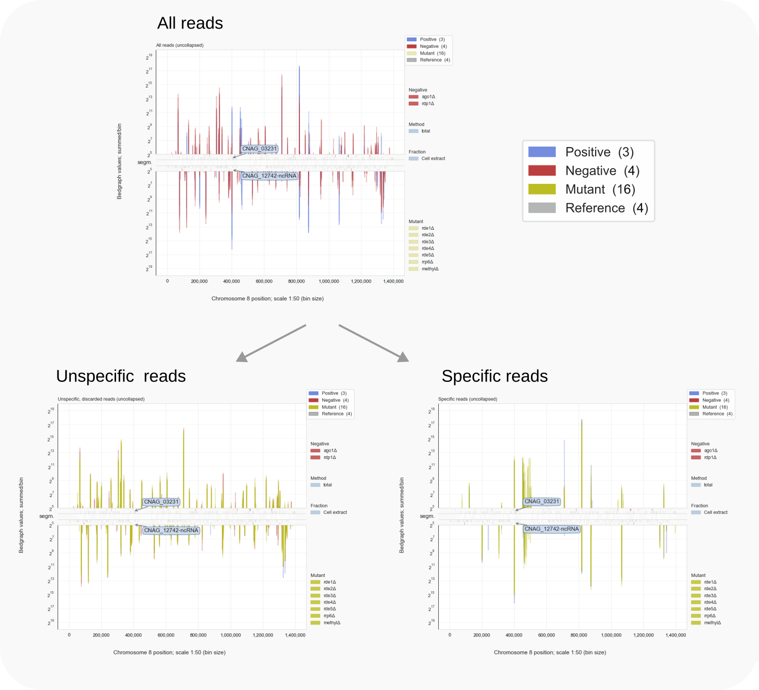
This command can be set to show uncollapsed (default) or collapsed data (with type option -t1), and with -r for a chromosomal region defined by two coordinates. A particular display window can be chosen (option -w), but normally the default sequence is shown: first a display of all reads, then of filtered, unspecific reads and last, a third window with the remaining, specific reads. To choose from different sets of samples use option -s.
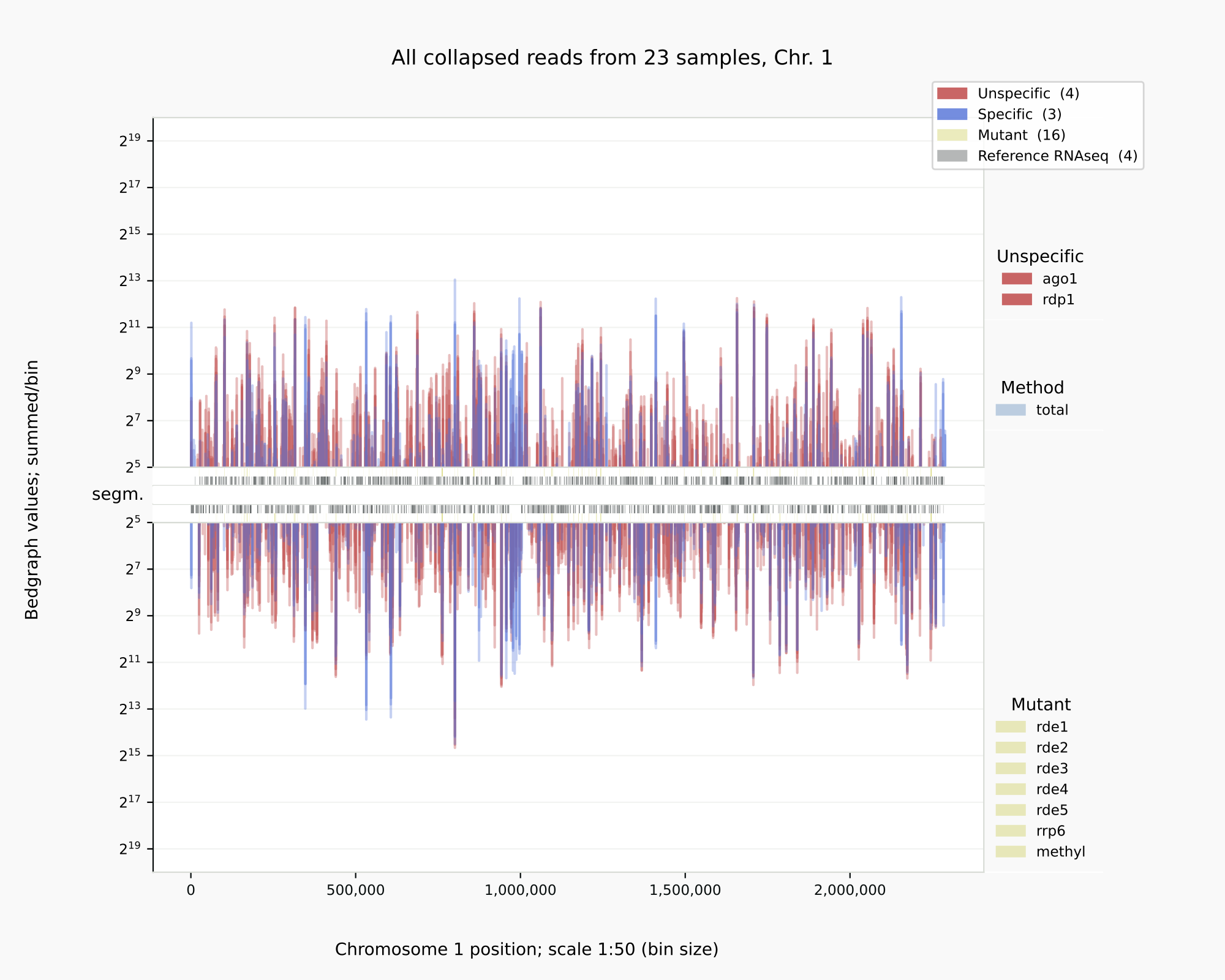
Specific reads for the positive controls and mutants [13] with
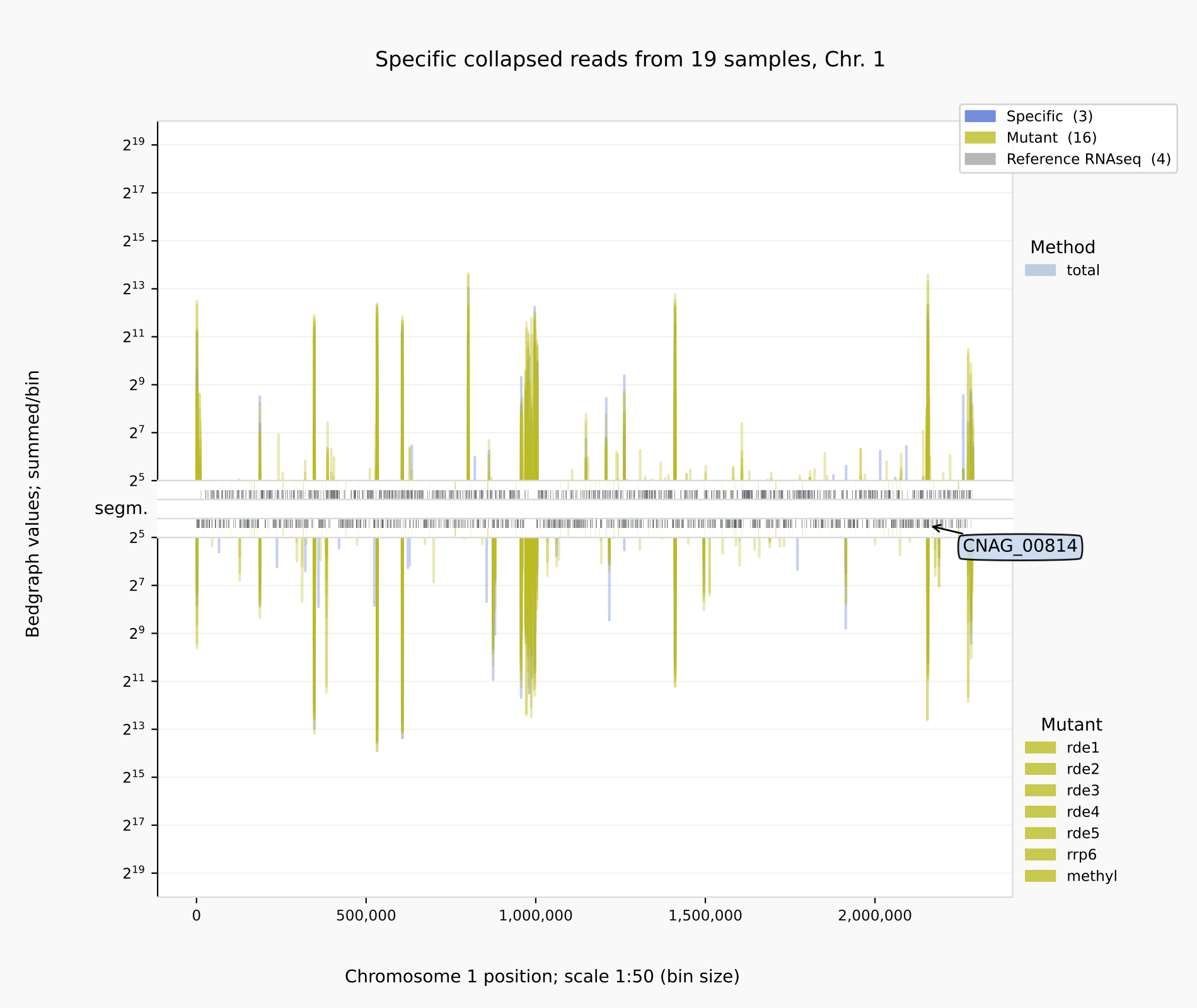
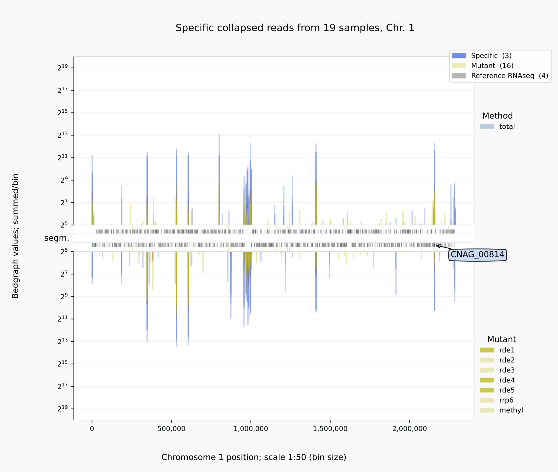
coalispr showgraphs -c1 -t1 -w4. The relative amounts of siRNAs were reduced in the cDNA libraries of mutants rde1, rde4 and rde5 (right).
Below is illustrated how bedgraph representations differ between a genome browser like IGB (left) and Coalispr (four panels on the right, the top two from a run with command showgraphs -c1 -w4 and the bottom two from a run in a separate terminal with options -c1 -t1 -w4). They provide complementary insights. The 1 nt resolution of IGB allows detection of precise boundaries, while Coalispr provides the ability to quickly load all samples and compare them in one go. For example, it is easy to enlarge the genomic context of the transposon with the CNAG_00814 transcript (with the ‘Zoom rectangle’ tool draw a box inside the middle segm. bar spanning the region of interest around 2,500,000) [16]. In the upper section uncollapsed data traces with predominant anti-sense peaks in comparison to the collapsed data below [15] are shown. From one Coalispr display, different images can be output, depending on which highlights and traces have been toggled to be shown: both kinds of representation reveal a difference between various mutants, with rde1, rde3 and rde5 signals matching those of the negative control background (red); the rde2 signals are halfway the background and those for the wild type (blue), while the rrp6 profile deviates in both signal height and coverage. Sharp troughs in traces displayed by Coalispr match introns in the genome browser, showing that RNAi is mostly directed at spliced RNA transcripts, contrary to the model proposed by [Dumesic-2013] et al. [17].
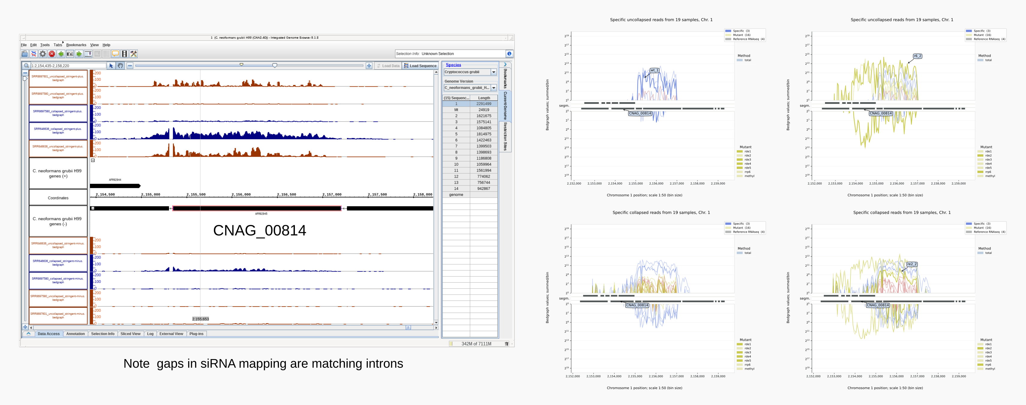
Intron skipping siRNAs against CNAG_00814 at resolution 1:1 (IGB image, left) vs 1:50 (right) [13].
showcounts
Information obtained by counting reads can be visualized using scripts [10] shipped with Coalispr and called by the coalispr showcounts command. The scripts provide a quick insight in the properties of the sequenced libraries:
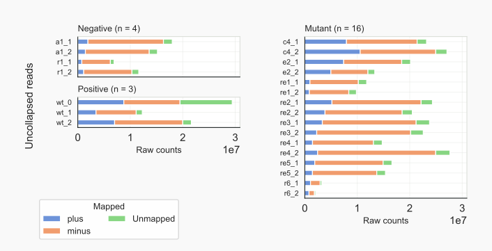
Input counts. With parameter -rc raw input counts will be displayed, split over strands (PLUS, MINUS) while unmapped reads are shown [18]. This gives a quick overview of differences between the libraries analyzed. The type of reads shown (TAGCOLL or TAGUNCOLL) can be chosen as well as the grouping of libraries (group option -g) according to either CATEGORY (UNSPECIFIC, SPECIFIC, MUTANT; default) or the METHOD used to prepare the sequenced RNA [20]. Grouping per category will, for input counts, also show unused DISCARD samples; these can be omitted by including the exclude option -x 1.
The abundance of reads mapped to the minus strand in especially unspecific or total sRNA preps of Cryptococcus (de)neoformans is very noticeable: their rDNA is encoded on a negative strand (that of Chromosome 2) [21].
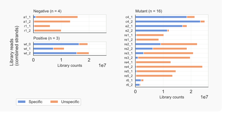
Library counts. Total library counts, for specific vs. unspecific reads can be diagrammed using parameter -lc, and grouped via option -g. Data per strand can be shown with stranded option -st (COMBI, default; MUNR, CORB). Based on the cigar string, alignments can be evaluated; only fully matching sequences (with or without one intron-like gap) are counted; all other alignments are skipped (SKIP), but their number logged to a separate file. Change scales of count numbers or show difference with unspecific reads based on log2 values with option -lg.
These figures highlight the variability between libraries and reveal the over-representation of unspecific reads in samples where production of expected siRNAs has been affected: compare mutant (category MUTANT) libraries with those of the negative (UNSPECIFIC) and positive controls (SPECIFIC). For C. neoformans H99, this suggests that not many genuine siRNAs are present in mutants rde1, rde4, or rde5.
Length distributions. In fungi like Cryptococcus, siRNAs range from 20-24 nt and tend to have a U (T in cDNAs) as the 5’ nt. The length-distribution option -lo forms an overview of the total of all library-reads split according to length of the reads and their starting nucleotide. Specific reads are compared to unspecific reads. One can choose to get information for all library (LIBR) reads, cDNAs (COLLR), or other reads, like those mapping to sequences used to genetically manipulate the strains (CHRXTRA) [18]. Sequences can be added, via ADDGDNA in the configuration file, when these are missing from the used reference genome, so that homologous library reads or cDNAs can be accounted for [19]. Reads that map to a unique (UNIQ [4]) locus, or those that can be aligned at multiple loci (MULMAP), can be selected by means of an extra option -ma.
The spread of intron lengths (number of mismatching N s skipped to align a read conforming to intron definitions in STAR; INTR) in LIBR or COLLR can be displayed. For this, limits on the x-axis can be set via MINGAP, MAXGAP, INTSKIP, with labels shown after each INTGAP. Use option -ld to display the length-distributions of separate libraries for the set kind of reads (change with -k). Group libraries with -g, select mapping type with -ma, or show stranded data with -st in combination with -ld or -lo.
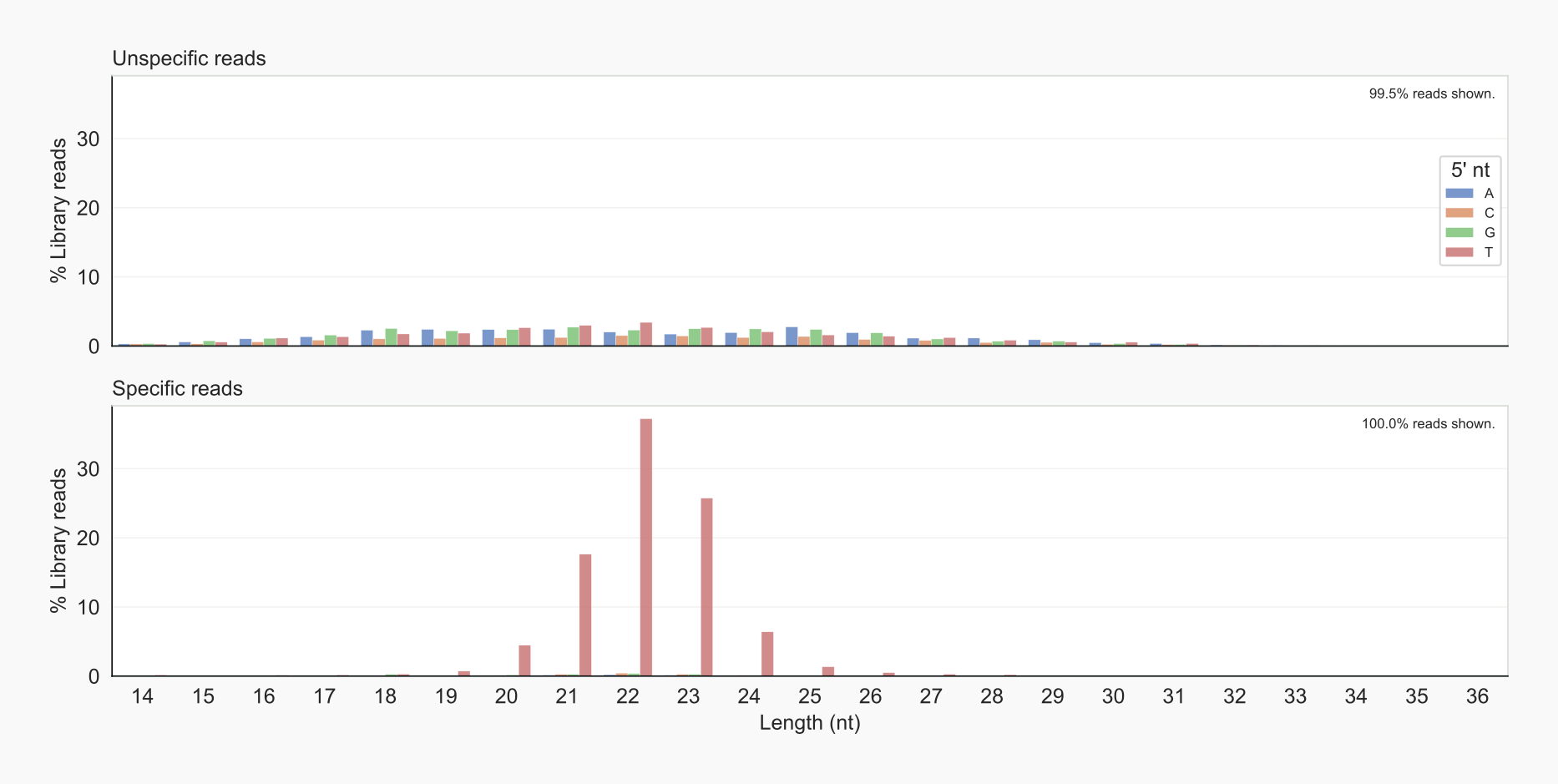
Overview of length distribution of specified reads.
coalispr showcounts -lo 1.By default, figure titles are turned off with the notitles option -nt 1; the relevant information is retained in the window title and included in the file name when saving an image. Use -nt 0 to display figure titles.
As expected, unspecific reads are characterized by an almost homogeneous distribution of fragment lengths, while specific reads peak around 21-23 nt for cDNAs beginning with a T. These are also slightly enriched in the unspecific reads, maybe due to being unselected.
Diagrams of reads mapping to extraneous sequences [23] demonstrate that RNAi in strains is triggered upon introduction of foreign nucleic acids: siRNAs are formed against transcripts from bacterial origin of replication, cas9 and especially target CRISPR/Cas guide RNAs transcribed by means of an U6 promoter [Wang-2016].
Bin diagrams can display the distribution of reads, expressed as a percentage, over the counted segment, which has been split up in a number of bins as determined by the parameter BINS. The relative counts of a sample will be placed in bin 1 (the most upstream bin), 2, … BINS (the end bin). Segments that appear too short (i.e. less than the length of BINS * BINSTEP) will not be split and these counts are kept in bin zero (0). Percentages are relative to all counts in a sample.
region
The script called with coalispr region provides an insight into the length distribution and number of reads that are found in a particular region of the genome (say rDNA). After entering the chromosome name (with option -c), a dialog asks for inputting the region coordinates or these can be given directly with option -r (like with coalispr showgraphs -r). Option -st controls whether reads aligning to the PLUS or MINUS strand are analysed (default is both, COMBI). The samples to be counted can be set with option -s (by default the controls). The terminal provides feedback and count results are saved to count files and displayed as bar diagrams, which are automatically saved. For proper parsing of all options, place the -r option plus coordinates at the end of the command.
Tip
The -r and -c options work in an identical manner in coalispr showgraphs and coalispr region.
- Facilitate region analysis for chromosome
Kby: Run in a terminal
coalispr showgraphs -c K -w2.Zoom into the region of interest.
Register chromosome coordinates by clicking the x-axis label.
The output is shown in the terminal as
K:<region>.Highlight
<region>and copy withShift+Ctrl+C.
- Facilitate region analysis for chromosome
- Open another terminal for running
coalispr region -c K -s1 -st 1 -r <region> Paste
<region>withShift+Ctrl+V.
- Open another terminal for running
Retrieve a display of the same chromosomal locus with
coalispr showgraphs -c K -w2 -r <region>.
To reduce complexity, a limited number of categories are compared, which is set by option -cf. By default libary reads (LIBR) and collapsed, i.e. cDNA, reads (COLLR) are counted. The number of reads that were skipped because of mismatches or point-deletions are reported too. The collection of counters used for this function is defined by the constant REGCNTRS in the 2_shared.txt configuration file.
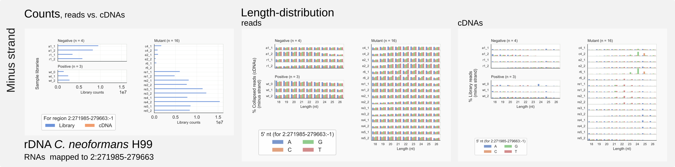
Minus strand counts for the C. neoformans rDNA unit on chromosome 2.
coalispr region -c2 -r 271985-279663 -st 3 -s2.Region analysis demonstrates that no reads are specially enriched among rRFs in Cryptococcus that would fit the siRNA binding pocket on Argonaute. Here, rRFs form a large but biologically uninformative background signal. When there is a large variability between libraries, this would undermine the possibility to normalise against rRNA background or the number of total mapped reads which contains a large but inconsistent fraction of unspecific reads that are mostly rRFs.
Other options are available, such as for inclusion of any unused (-x) or redundant mutant (-rm) samples as well as figure titles (-nt).
annotate
Count files generated with coalispr countbams can be compared to reference files and annotated with available gene information. For this, the annotation files GTFSPECNAM for specific reads and GTFUNSPNAM for unspecific reads are used according to the values for above constants in the experiment file (EXPFILE). With option -rf 1 annotations in GTFREFNAM for REFERENCE reads can be included as well, extending the processing time. The annotation files are the same as used in the displays created with coalispr showgraphs.
By default a count file for specific uncollapsed library reads (LIBR, ALL) is annotated; with library-choice option -l 2, the input will be a count file for cDNAs (collapsed reads, COLLR).
Annotated files are saved to OUTPATH (that is SAVEIN / OUTPUTS / EXP, normally the experiment folder in Coalispr/outputs/ in the work directory) and sorted on value in descending order. To keep annotated files organised according to genome position, turn the sort-value option off: -sv 0.
Other options are: -k 0 to change the kind of reads to unspecific; -st {1,2,3} to define strand-specificity for COMBINED (default), MUNR (-st 2) or CORB (-st 3); -ma {1,2} to select count files for UNIQ reads or multimappers (MULMAP). Count numbers can be formatted to their log2 value with option -lg 1 and output files can include unused samples by setting option -x 0.
For examples see the annotate-section in the tutorial ‘Mouse miRNAs’ or this paragraph in the tutorial ‘Cryptococcus siRNAs’.
groupcompare
Described above, the command coalispr showcounts -ld produces an overview of detected readlengths for mapped RNAs for each sample. By including option -g the grouping of samples can be set. With this command, all samples will be included separately in the figure.
To compare only a selection of samples according to a particular type, say, METHOD, FRACTION, CONDITION or GROUP (i.e. mutation) the command coalispr groupcompare -g might provide a cleaner view. This command generates a grouped bardiagram showing the average (MEAN or MEDIAN with option -av) with error bars for the standard deviation between the values for the samples in each group. After setting the major type for the comparison with the required group option -g, samples are selected according to available groupings still present among selected samples -s. With option -5e the start-nucleotide of reads to be examined can be chosen, while read length option -rl sets the minimal and maximal lengths of reads to be displayed. As for the coalispr showcounts command, specific views for strands (-st), uniq - or multimappers (-ma), or the kind of read (-k, SPECIFIC or UNSPECIFIC) can be generated; it is possible to include any unused (-x) or redundant mutant (-rm) samples, or show figure titles (-nt).
Note
Command coalispr groupcompare and grouping option -g will only be available if the experiment file, EXPFILE, describes various groups.
info

Settings vs. number of contiguous regions [13]
coalispr info -r2)This command provides information on the current session, like the setting for setexp (by default), memory-usage of the data in Pandas [25], the path to configuration files or Experiment file. The option -pV 1 opens a Parquet viewer to inspect files with binary data or counts. This viewer is embedded in the GUI.
The regions option -r helps to assess which parameter settings fit the quality of the data. One can vary a number of values for each parameter by editing the three parameter lists in 3_EXP.txt, namely UNSPECTST, UGAPSTST and LOG2BGTST [26]. The number of combinations to be tested in one run and thereby the time this takes, increases with the length of the list for each parameter. This because each combination is assessed against collapsed (TAGCOLL), and uncollapsed (TAGUNCOLL) data for both SPECIFIC and UNSPECIFIC reads. When previous output from coalispr info -r1 is present, the run halts unless the force option is set (-f 1); this will back_up the existing data file before writing the newly created data to disk.
For some chromosomes high thresholds can prevent detection of specific signals so that no regions are found [24]. Such empty chromosomes cannot be displayed with coalispr showgraphs by lack of bins with data.
Note
When the stringency of a parameter is too high, no reads can be marked as SPECIFIC, giving an empty array.
UNSPECLOG10. High signal-to-noise ratios allow for stringent separation of specific from unspecific reads. For this, use a large value for UNSPECLOG10. This parameter sets the exponent for the 10UNSPECLOG10-fold difference that defines the threshold when positive and negative reads overlap (see explanatory figure). With stringencies set too high, no specific peaks can be specified for a chromosome. Such a combination of settings cannot be used. In the settings figure, this is shown by an absence of region numbers (see panels with UNSPECLOG10 >= 1.0) [13].
UNSPECLOG10 values have not a big influence on the number of regions with unspecific reads (visualize with coalispr info -r3). That many more regions with collapsed reads are found relates to single reads in a library gaining more prominence [15].
In the configuration file, the list UNSPECTST contains the values for UNSPECLOG10 that are tested during coalispr info -r1
USEGAPS, UNSPCGAPS. Stringent thresholds can lead to gaps between peaks when counts for intermittent regions drop out not meeting the set cut-off levels. With USEGAPS a tolerance is set that creates a contiguous region of reads when its peaks are closer together than the gap-setting [27]. A low USEGAPS reduces the number of peaks that are taken together and results in a high number of regions with specified reads. When USEGAPS is set too high, sections are fused that represent separate regions, albeit relatively close together [26]. For defining segments used in the counting of unspecific reads, peaks are not fused; by default the gap (UNSPCGAPS) is kept minimal, i.e. equal to BINSTEP.
The values for USEGAPS tested during coalispr info -r1 are in the list UGAPSTST of the configuration file.
LOG2BG. To minimize the number of regions with a very low level of specified reads, the signals need to be higher than a threshold of 2LOG2BG [26].
For values of LOG2BG that are tested during coalispr info -r1, see/edit the list LOG2BGTST in 3_EXP.txt
test
During development this module helped to quickly test functionality by means of predefined showgraphs, countbams, region, info -r1 or annotate commands. For commands countbams or annotate the kind (-k) of reads to be analysed can be set. To give an idea of how these sections perform, coalispr test -tp also writes profiling information to the terminal using profilehooks. To activate the test command set TEST in coalispr.resources.utilities.py to True.
GUI
A Graphical user interface (GUI) can be called from the command line by coalispr_gui . The GUI can be used to access above commands directly, with all available options accessible on the run tab. Required options are in red, help for each option is shown by mouse-over on the labels. General help for the command is on the help tab. Two other other tabs provide access to (binary) files to check the generated data and counts.
The GUI is based on Tkinter, shipped with Python, and uses an external module, ttkbootstrap, for the look and feel, applying a colour scheme based on the Coalispr logo.
Note
Because Tkinter is required for running coalispr_gui, the BACKEND is set to ‘TkAgg’ as the default in the SHARED configuration file. This also functions with coalispr from the command line (CLI).
The run tab opened via init shows the current experiment settings and chromosomes. A Choose work environment button opens a file dialog to browse to and pick the directory for placing the Coalispr folder. Do this in preparation of changing between experiments or to initiate a new session.
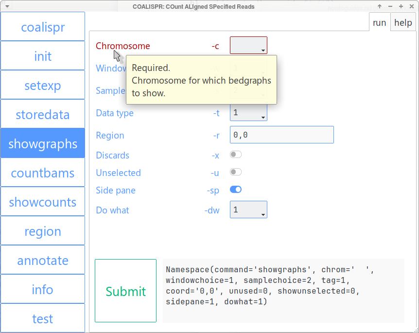
coalispr_gui with run tab for command coalispr showgraphs open.
Submit button passes the displayed Namespace ascoalispr showgraphs function.Note
Output from functions/commands run by coalispr_gui will be displayed on the command line (that is, the terminal from which the GUI has been started). Also dialogs and requested input use the command line (The GUI will become unresponsive when waiting for user input on the command line). For some commands - as indicated by the tooltip on the SUBMIT button after mouseover - the program will restart when the commands have run. Completion of such commands alter the state of the program and this new state is only assessible by a restart of the GUI. For example, with setexp a novel configuration needs to be loaded, or after storedata or countbams downstream commands become feasible but need access to the newly acquired information.
Troubleshooting
Coalispr has been developed and tested on a computer operating with Slackware linux. Hiccups in other environments can be expected. The program is run from the command-line which can also show errors or warnings which interfere with the feedback provided by Coalispr. Some of the messages are not from the program but relate to the context of running Python and Matplotlib and can be removed by changing a configuration setting.
When the program is not behaving, please consider:
Log files
To help solve problems, error messages generated by Python are logged, including some feedback on commands and their parameters. The log files (run-log.txt, LOGFILNAM) are stored here:
<Work-environment>/ Coalispr / logs / <EXP> / run-log.txt
that is, in the logs (LOGS) directory in the Coalispr folder that was set up in the work environment by coalispr init, and placed in a sub-folder with the name of the current experiment (EXP, chosen via coalispr setexp).
Maybe the log files can give an idea where the error comes from and how it can be solved. Please, include the relevant section of the run-log.txt when reporting an issue at the Coalispr repository.
Backends
BACKENDs are the programs matplotlib uses to present a graphical users’ interface (GUI). You will see that this setting determines the look and feel of displayed graphs (with showgraphs, showcounts, region or info. A nice backend is “QtAgg”, but when many samples are analyzed some showcount options can lead to a crash with:
ICE default IO error handler doing an exit(), .. errno = 32
Errors or warnings with “GTK4Agg” can also occur, like:
Warning: Attempting to freeze the notification queue for object
GtkImage[0x5e7f690];
Property  notification does not work during instance finalization.
lambda event: self.remove_toolitem(event.tool.name))
In such cases change BACKEND in the EXPTXT to, say, “TkAgg” or “GTK3Agg”.
Because TkAgg is needed as BACKEND when running coalispr_gui this is now the default and the PyQt-dependency for “QtAgg” has been removed as a requirement for running Coalispr.